For Students
For Students
Learning Online Orientation
If this is the first time that you are taking an online course, then we would strongly urge you to work through the pages that follow here. We'll go through how our online courses work, what technologies are used, proctored exams, how to be successful online, and where to go for help when you need it.

Math & Stat Reviews
Check out this section if you need a refresher on Algebra, Basic Statistical Concepts, Calculus, and more! Make sure to consult the course prerequisites to know what knowledge is expected upon entering a course.

Ethics and Statistics
At Penn State University, academic integrity is a critical ingredient in any program wether it be in residence or online. The Penn State Values were developed to embody the values that we hope our students, faculty, staff, administration, and alumni possess.
Learning Online Orientation
Learning Online OrientationWelcome to the Orientation Materials for the online courses associated with the Department of Statistics!
If this is the first time that you are taking an online course, then we would strongly urge you to work through the pages that follow here. We work hard to ensure that your learning experience is as positive for you as possible and we hope that the information and contacts that you will be introduced to in this orientation will help to point you in this direction.
Objectives
- Be able to describe the general nature of how the online courses are designed and the online course environment.
- Understand the role of students in an online course and what is expected from them.
- Be able to list a range of technologies that are used in association with our online courses and be able to assess whether the computer setup that they will be using is able to handle how materials are presented and interactions with others.
- Be able to list the various statistical software packages that are used as part of the online courses be able to describe how to obtain a copy of this software so that it can be installed before classes begin.
- Be able to list a range of resources and services that are available to Penn State students.
- Know who to contact when you need additional information about the program or about learning online at Penn State.
- Know who to contact when you need technical assistance.
Begin by reading through the pages that follow in this module. Follow the links that are presented so that you can check the various technology requirements on your own computer and make note of the different services that are described.
There will be a short quiz at the conclusion of these materials.
If you have any questions as you go through this Orientation, please feel free to contact John Haubrick, instructional designer & teaching faculty, Department of Statistics.
O.1 How do the online courses work?
O.1 How do the online courses work?The activities in the online courses offered by the Department of Statistics are found in two different but connected locations. The course administrative functions such as announcements, grade book, homework assignments, quizzes, and exams are all accessed from within Canvas, Penn State's learning management system. Here is a link to a Canvas Overview Video for Students if you want a sneak peek at how Canvas works. Other useful documentation for using Canvas can be found in the Canvas Student Guides. Lesson materials such as lecture notes, examples, animations, movie or audio clips, or other interactive pieces that are needed to help drive an important concept home are found on the companion course materials website.


Each course companion website intends to provide students with information, examples, images, formulas, or code that supplements what is presented in the required readings or in the instructor's Canvas course space. Wherever possible we try to make these interactive when this helps to aid understanding. In general, our notes strive to provide a rich narrative, liberally enhanced with graphics and augmented with video where appropriate. Where other online programs may base their online materials on recorded lectures, our approach intentionally promotes the use of short video segments that are embedded with our online materials for the purpose of presenting specific concepts, sharing worked examples, or responding to student questions. Our online material websites also include a search tool and a printer-friendly option, and all formulas and equations are rendered using MathJax (more on this later!).
FAQs
Click on the frequently asked questions below to view the answers.
An important aspect that all of the online courses include is interaction - interaction with the instructor as well as interaction among students. The course's email, discussion forums, and live chat are tools typically used for these interactions, however, many instructors take advantage of other video or interactive whiteboard types of communication tools outside of the course management system where they can work with students as a group or individually.
In Canvas you can find out who your classmates are by selecting the 'People' link on the left. Each course typically starts off with an introductory activity. Take advantage of this to introduce yourself to your instructor and your fellow classmates. Later on, in this orientation, you can follow the tips to update your profile in Canvas by clicking on your Account > Profile and adding information to this page.
Want to know more about your instructor? Start with the Online Instructors page or send them an email.
The course schedule is published along with the syllabus at the beginning of the semester by the course instructor. Depending on the course, the flexibility of the course schedule varies, but in general, our courses are pretty well packed with readings, homework, quizzes, exams, etc. We work hard to maintain the policy of Penn State University and the Department of Statistics that all of our online courses are equivalent to what would be taught in the residence course section on campus and we take this curriculum integrity issue seriously.
Our online courses all follow the same academic calendar as the rest of the university, with perhaps a few changes because it is online. And, all of our courses are cohort-based. This means that all the students start at the same time and work through the lessons at the same time, with the instructor opening and introducing perhaps a couple of lessons at a time. Our courses are not open-enrollment oriented where everyone is on their own studying at their own pace. This would make discussions problematic and the role of the instructor nearly impossible trying to direct your attention and answer questions from all directions! Also, given the wide array of time zones that our students represent, nearly all of the activities in our courses are asynchronous. Instructors may establish times for office hours that are held in an online meeting room, (recorded for those that can not attend) or an instructor may want students to present work to the class, but in general, most of the work and interaction takes place individually through email, discussion forums and other methods that do not require everyone to log in at a specified time.
The pace and approach to courses are very similar to how things are taught face-to-face. In fact, some of our online instructors are teaching the same course on campus. However, this being said, and because this is online and we realize that our online students are typically returning adult professionals with full-time work and family responsibilities, our instructors try their best to make accommodations. For instance, we've come to realize that for many the majority of the discretionary time you have to apply to coursework has been on weekends. Therefore, a Friday deadline for homework is problematic for many. We found that shifting due dates to Sunday night or Monday works better for most. Again, when something comes up, travel, medical, or other issues, that might impact your ability to meet deadlines, whenever possible reach out to your instructor ahead of time.
This is a good question, and of course, you might expect the answer, "It depends". Well, it does depend. It depends on what background understanding you bring to the course. And it depends on the course. Some may involve a lot more work for you, whereas other courses may involve much more difficult concepts or methods.
To help you answer this question, take a look at the results displayed in the pie chart (right). Every semester we administer a Mid-Semester Survey in each of our courses as a means of monitoring the perceptions of our students and providing an opportunity for feedback. These are the results combined across all of our MAS courses during the Summer 2018 semester asking how much time students spend on their course. The Graduate School guidelines at Penn State state that a student should be expected to spend 3 hours outside of class for every course credit. So, for a 3-credit course, one would expect to spend 9 hours on reading, homework, study, etc. Taking this into account, the pie chart shows us that our students are reporting that we pretty much meet this standard. For instance, 40% of students reported spending 4-6 hours on a course, and 39% of students reported spending 7-9 hours per week on a course. In the long run, we work to ensure that our courses are rigorous without being impossible and that what you learn is of lasting value.
Each course includes an assessment plan which is published as part of the course syllabus. Deadlines for each of these assignments are given in the course schedule. By the way, all of the course due date times are US Eastern Time (the Canvas timestamp) - not for each of your time zones. The deadline time is set so the grading and feedback process can begin. Keep up with the course schedule. If you get behind it is a real chore to catch up! This would be true in a face-to-face class as well.
All assessments are submitted in Canvas. Lesson quizzes are mostly multiple choice but could include T/F or essay-type questions as well. Sometimes it might be necessary to write out an assignment by hand. In these cases, students will need access to a scanner that would produce a .pdf of their work which could then be submited to your Assignment or Quiz in Canvas.
Whereas homework and labs are open until they are due, mid-terms and exams are available to be taken by students during the pre-established time frame. For instance, if a 90-minute mid-term is open beginning Thursday to Sunday, then students will need to find a 90-minute time slot somewhere in this time frame that they can complete this exam. Additionally, some courses have exams that are required to be proctored. For more information about proctored exams read What is a Proctored Exam?
Because these courses are online we will be using various technology tools. We will tackle this in the next section...
O.2 What technology is used?
O.2 What technology is used?In our online statistics courses, you will use a variety of technologies to facilitate the learning process.
The following sections highlight just a few of these technologies. Visit the Technology Tutorials on this site for more information on the technology used in our courses.
Other Resources
- Canvas Orientation
Canvas orientation course created by World Campus. - Penn State IT Connect to Tech Student Guide
Penn State's main resources for tech available to students. - Statistical Software page
Stat Department list of software needed for each course. - Technical help and support resources
List of contact information for various technical support services
Technical Requirements for Online Courses
Technical Requirements for Online CoursesRecommended Technical Requirements for "Frustration Free" Computing
View our World Campus Technical Requirements page to see the minimum technical requirements for our courses.
To review minimum technical requirements for individual statistical software packages, please visit the technical support pages of the individual vendors. See the Statistical Software page on the Statistics Department website.
Students are strongly encouraged to download, install, and test computer and browser requirements prior to the beginning of classes.
Courses with Proctored Exams
For courses using Honorlock you must meet the following technical requirements.
Honorlock System Requirements
See Honorlock's Minimum System Requirements page.
Reaching Honorlock 24/7/365 Support
- Phone: 1 (844) 243-2500
- Email: support@honorlock.com
- Live Chat: Click on the live chat link located at the bottom right corner of your Canvas exam page
- Honorlock support: Click on the link at the top right-hand corner of your Canvas exam page
Learning Management System: Canvas
Learning Management System: CanvasThe course administrative functions such as announcements, gradebook, homework assignments, quizzes, and exams are all accessed from within Canvas, Penn State's learning management system.
There are numerous resources we recommend you review if this is your first time using Canvas.
Canvas Resources
Take a Screen Capture
Take a Screen CaptureIn the online environment, being able to capture graphs, images and equations is an important skills for assignments, discussion forums and even troubleshooting issue with your instructor to the help desk.
Most new operating systems come equipped with some sore of screen capture tool. Here are the basic ones.
Windows Windows
Using Keyboard
- PrtScn: Another option is to use the print screen ("PrtScn") function which will copy your entire screen, then paste it into Word and crop down to only the necessary part of the screen.
- SHIFT + S: (Windows 10 only)
Using built-in tool
- Snipping Tool: Computers with Windows Vista and later will have a snipping tool. This will allow you to select a portion of your screen. Then, you can copy it and paste it.
macOS macOS
Using Keyboard
- ⌘ + shift + 4: This will allow you to select a portion of your screen. By default, this saves your screenshot as a graphic
Using Built-in tool
- Grab: This tool will allow you to capture, the entire screen or just a selection.
Once you have your image you can then upload it to Canvas or add it to your document.
Uploading an image to a Canvas Forum or Quiz
As a student in our online STAT courses, you may have to upload an image to a discussion, quiz, or assignment in Canvas. Canvas provides a way to upload directly from their rich content editor.
View the step-by-step procedures in the Canvas documentation.
How do I embed images from Canvas into the rich content editor as a student?
Working with Images in Documents
Cropping a Picture in Word
There are times when you have to crop your screenshot to only show certain parts of the image in your document.
O.3 What is a proctored exam?
O.3 What is a proctored exam?Proctored Exams
Some courses require the use of Honorlock proctoring software to protect academic integrity during certain course activities. While active, this software uses your computer's webcam and microphone to record video and audio, while other technology monitors your activity, including your screen and web navigation.
You will need a computer (not a phone or tablet) with a microphone and webcam and one of the compatible operating systems listed in Honorlock's Minimum Requirements table. Additionally, you will need to use Chrome and download the Honorlock Chrome Extension.
The information collected by Honorlock is confidential and will only be used for legitimate academic and educational purposes. For further information, see the Penn State Honorlock privacy statement and Honorlock’s Student Data Privacy & Security information.
Resources:
If you have any technical issues or questions, please reach out to Honorlock support via live chat on the Honorlock support page or through the exam itself.
O.4 How can I be successful?
O.4 How can I be successful?OK, so you now have the technology all in place, your browser and plug-ins working and a reliably fast internet connection. This is good but it is just a start! There is more to learning online than just the technologies!
We want you get to most out of your online learning experience. So, we have put together a list of 'Tips & Suggestions' that have been gathered from research and our own experience working with students. We want you to listen to interviews with students who share their own advice based on their personal experiences and what they have to say about how they organize their time so that they can complete all of the necessary tasks and activities for a course.
Read through these suggestions, watch the video and then make a personal plan for an approach that will help you make the most of your online learning experience!
Tips & Suggestions
- Pay close attention to the due dates of the assignments and check the Syllabus regularly in case changes have been made by the instructor!
- Plan ahead and plan well. Do not put off quizzes or assignments till the last minute! Courses in statistics are challenging and these courses are no different. If you begin to fall behind it will be very difficult to catch up!!
- Check your e-mail regularly, but be patient while waiting for responses.
- Communicate with your instructor and/or classmates by e-mail, message boards, chat rooms, Instant Messenger, or phone. Subscribe to discussion forums so that you get notified if there is a post!
- Use courtesy in online communication and deal with conflict with respect.
- Evaluate your own progress by the course objectives and assignments, and regulate your own study pace based on this evaluation. Talk to your instructor if you encounter a problem.
- Participation is important to your learning experience in an online learning environment, so be confident in making contributions. Don't be afraid of making mistakes!
- Identify a way of taking notes you would prefer: use Word, online journal/Web logging, note-taking software, bookmarking the Web sites important to you, or any method that works well for you.
- Be aware of the resources for HELP available: your instructor, the Outreach HelpDesk, Outreach Student Services, Canvas Help, or a librarian.
- Always check the file size when you try to upload a file to share. The bigger the file size, the more difficult it may be to upload and download.
- In addition to becoming familiar with the online learning environment, pay attention to the physical learning environment around you - try to arrange everything ergonomically in your learning space.
- Be sure to always display appropriate "Netiquette". Netiquette covers not only rules to maintain civility in discussions but also special guidelines unique to the electronic nature of forum messages. View Penn State's Earth and Mineral Sciences faculty development resource on 'Netiquette'.
Ask GOOD Questions!
Communicating back and forth with your instructor and classmates using email or discussion boards can be frustrating because of the back and forth nature of trying to find out specifically what you need to know. For this reason it is important to ask questions that have enough information so to ensure that you will efficently get a helpful answer in return.
- Be Specific! For instance, if you ask, "I just don't get problem #4, can anyone help me?" - this is pretty general and I am sure potential respondents are saying, "Where do I start?!" Instead, add more specific details to help your helpers help you more efficiently. If the question posted was, "I am gettting a different value for the standard error and here are values that I am using. Can anyone see what I am doing wrong?"
- Capture Your Screen! They say a picture is worth a thousand words - so you might as well take advantage of this! Rather than explain, show what you see when you can. You can then either embed this in your message or add it as an attachment. This can save you are your instructor lots of time!
O.5 What resources are available?
O.5 What resources are available?Penn State provides a host of resources to every Penn State student. Here are some pages that we think might be of particular interest to our online students.
Penn State Information and Resources
The pages that follow provide specific information that you can skim through quickly. Perhaps something will catch your eye that you might want to investigate further.
In any course, whether it is face-to-face or online, as a student of The Pennsylvania State University, you are required and expected to understand and accept our policies on academic integrity and plagiarism. While you may have read this information in other courses, you are encouraged to re-read it.
Academic Integrity
Academic integrity is the pursuit of scholarly activity free from fraud and deception and is an educational objective of this institution. Violations of academic integrity include but are not limited to, cheating, plagiarizing, fabricating of information or citations, facilitating acts of academic dishonesty by others, having unauthorized possession of examinations, submitting work of another person or work previously used without informing the instructor or tampering with the academic work of other students. At the beginning of each course, it is the responsibility of the instructor to provide a statement clarifying the application of academic integrity criteria to that course. A student charged with academic dishonesty will be given oral or written notice of the charge by the instructor. If students believe they have been falsely accused, they should seek redress through informal discussion with the instructor, department head, dean, or campus executive officer. If the instructor believes that the infraction is sufficiently serious to warrant referral of the case to Judicial Affairs, or if the instructor will award a final grade of "F" in the course because of the infraction, the student will be afforded formal due process.
For this and every course, you are required to read and abide by Penn State's Academic Integrity Policies. Each course syllabus contains a statement similar to the one below with links to the Eberly College of Science's policies governing Academic Integrity:
All Penn State policies regarding ethics and honorable behavior apply to this course. Academic integrity is the pursuit of scholarly activity free from fraud and deception and is an educational objective of this institution. All University policies regarding academic integrity apply to this course. Academic dishonesty includes but is not limited to, cheating, plagiarizing, fabricating information or citations, facilitating acts of academic dishonesty by others, having unauthorized possession of examinations, submitting work of another person or work previously used without informing the instructor or tampering with the academic work of other students.
For any material or ideas obtained from other sources, such as the text or things you see on the web, in the library, etc., a source reference must be given. Direct quotes from any source must be identified as such.
All exam answers must be your own, and you must not provide any assistance to other students during exams. Any instances of academic dishonesty WILL be pursued under the Eberly College of Science Academic Integrity Policies concerning academic integrity.
The Eberly College of Science Code of Mutual Respect and Cooperation embodies the values that we hope our faculty, staff, and students possess and will endorse to make The Eberly College of Science a place where every individual feels respected and valued, as well as challenged and rewarded.
To learn more about specific scenarios such as: How to avoid plagiarism? Academic integrity issues that may arise when collaborating with a group? and others, visit Penn State's Academic Integrity Training. You can test your understanding of these issues and those that score 80% or better will earn a certificate.
Use the Penn State Libraries!
As a Penn State student enrolled through World Campus, you have a wealth of library resources available to you — just like on-campus students! Please review the World Campus and Distance Researchers page on the library site. Eligible users include currently enrolled or employed Penn State faculty, staff, and students in good standing who do not have access to a Penn State campus.
As a registered user of Penn State Libraries, you can...
- search for journal articles (many are even immediately available in full-text);
- request articles that aren't available in full-text and have them delivered electronically;
- borrow books and other materials and have them delivered to your doorstep;
- access materials that your instructor has put on electronic Library Reserves;
- talk to reference librarians in real time using chat, phone, and e-mail;
- ...and much more!
For additional information on using the Library as a World Campus student check out the following two flyers.
- Using the Penn State Libraries System
- How Penn State World Campus Students Can Request Library Materials
Library Contact:
Denise Wetzel
Science & Engineering Librarian
dawetzel@psu.edu
Statistics (Mathematical) Library Research Materials
Research or Subject Guides
Research guides help you find high-quality information and are created by librarians who are subject specialists in a wide array of disciplines. Search the research guides by keyword or use the alphabetical list to find the appropriate guide.
SAGE Resarch Materials
SAGE's Little Green Books, Methods Map, and Methods lists are all now available to all Penn State students for FREE! This includes the famous series, Quantitative Applications in the Social Sciences. This entire series is available on SAGE Research Methods, with additional tools across the site to filter your search on just these titles.
To access these SAGE Research Materials, go to the Penn State Libraries > click on the Databases tab > select 'S' > then click on the SAGE Research Methods Online link:

Penn State has been successfully offering education at a distance since 1892. One big reason for this success is because of the work of the folks in Student Services. From financial aid to technology support to career services, students are all encouraged to take advantage of the vast expertise they have gained over the years. They have recently received recognition for their work with students in the military. If you have not logged into your World Campus portal, follow the link to find out how. Penn State's World Campus has a variety of different services related to learning online that at one time or another, you may want to take advantage of.
Besides the help you may have received in getting admitted to a program, registering for courses, and technical support once your course gets started, there are also support services for students that you might not be aware of. These include:
- Financial Aid, Scholarships, and other benefits
- Support for Students in the Military
- Support for Students with Disabilities
- Career Services
Do you know how to defer loans you do have while you are a student? First, it is important to know that you have to be at least a half-time student in order to be loan eligible. And, once you have a loan it is important to demonstrate satisfactory academic performance, i.e., completing a course with a passing grade or your opportunity to obtain future aid may be in jeopardy!
World Campus provides a Student Portal that has links to help you answer all of your questions. The screenshot below of this portal points to some of the important links to check out!
Resources
There are a handful of valuable resources that every student will want to take advantage of while they are at Penn State including your account profile, Canvas, Office 365, Zoom, web publishing, software, and others. This page offers you a quick listing of services to check out!
When is the first day of classes? What does the drop/add period end? The Penn State calendars are a page that every student visits at one point or another!
O.6 Summary
O.6 SummaryThe Department of Statistics is proud to be able to offer these opportunities to learn online to individuals who otherwise might not be able to take advantage of taking a course or getting an advanced degree. We hope that the approach that we take will help you build your understanding and experience base in positive ways.
Having worked through this Orientation module you should now have a good idea as to how our online courses are delivered and the role that students play throughout the semester. Being all online you should understand that there are a number of technologies and internet resources that will be central to your success with the program. As a result, you should see the need to check the computer setup so that you have all hardware, software, and internet connection in place before any classes start. If you have any questions about any of this technical information, please do not hesitate to reach out to the contacts listed within the orientation.
Also, you should know that once you get your PSU Access Account userid, there are a host of resources available to all Penn State students, this includes through World Campus. Take advantage of these!
And, finally, if you have any questions about our courses, your program of study, or the technology, please do not hesitate to contact someone here at Penn State, in the Department of Statistics, or at one of the various Help Desks online.
Quick Tutorials
You will notice a 'Quick Tutorials' section of the website that follows this Orientation. These quick tutorials focus on some of the specific applications that are either used regularly in our online courses or tools or methods that we think will come in handy. Check them out! They are organized in terms of:
Math & Stat Reviews
Math & Stat Reviews
Algebra
Knowledge of the following mathematical operations is required for STAT 200:
- Addition
- Subtraction
- Division
- Multiplication
- Radicals (i.e., square roots)
- Exponents
- Summations \(\left( \sum \right) \)
- Factorials (!)

Basic Statistical Concepts
These review materials are intended to provide a review of key statistical concepts and procedures. Specifically, the lesson reviews:
- populations and parameters and how they differ from samples and statistics,
- confidence intervals and their interpretation,
- hypothesis testing procedures, including the critical value approach and the P-value approach,
- chi-square analysis,
- tests of proportion, and
- power analysis.

Calculus
It is imperative that you have a working knowledge of multidimensional calculus as a prerequisite.
This includes:
- differentiation,
- integration,
- series,
- limits, and
- multivariate calculus.
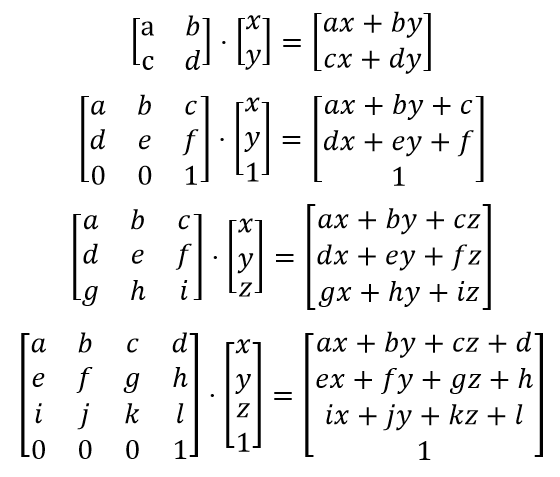
Matrix Algebra
Students who do not have this foundation or have not reviewed this material within the past couple of years will struggle with the concepts and methods that build on this foundation.
Algebra Review
Algebra ReviewKnowledge of the following mathematical operations is required for STAT 200:
- Addition
- Subtraction
- Division
- Multiplication
- Radicals (i.e., square roots)
- Exponents
- Summations \(\left( \sum \right) \)
- Factorials (!)
Additionally, the ability to perform these operations in the appropriate order is necessary. Use these materials to check your understanding and preparation for taking STAT 200.
We want our students to be successful! And we know that students that do not possess a working knowledge of these topics will struggle to participate successfully in STAT 200.
Review Materials
Are you ready? As a means of helping students assess whether or not what they currently know and can do meets the expectations of instructors of STAT 200, the online program has put together a brief review of these concepts and methods. This is then followed by a short self-assessment exam that will help you determine if this prerequisite knowledge is readily available for you to apply.
Self-Assessment Procedure
- Review the concepts and methods on the pages in this section of this website.
- Download and complete the Self-Assessment Exam.
- Review the Self-Assessment Exam Solutions and determine your score.
Your score on this self-assessment should be 100%! If your score is below this you should consider further review of these materials and are strongly encouraged to take MATH 021 or an equivalent course.
If you have struggled with the methods that are presented in the self-assessment, you will indeed struggle in the courses that expect this foundation.
Note: These materials are NOT intended to be a complete treatment of the ideas and methods used in algebra. These materials and the self-assessment are simply intended as simply an 'early warning signal' for students. Also, please note that completing the self-assessment successfully does not automatically ensure success in any of the courses that use these foundation materials. Please keep in mind that this is a review only. It is not an exhaustive list of the material you need to have learned in your previous math classes. This review is meant only to be a simple guide of things you should remember and that we build upon in STAT 200.
A.1 Order of Operations
A.1 Order of OperationsWhen performing a series of mathematical operations, begin with those inside parentheses or brackets. Next, calculate any exponents or square roots. This is followed by multiplication and division, and finally, addition and subtraction.
- Parentheses
- Exponents & Square Roots
- Multiplication and Division
- Addition and Subtraction
Example A.1
Simplify: $(5+\dfrac{9}{3})^{2}$
\end{align}
Example A.2
Simplify: $\dfrac{5+6+7}{3}$
\end{align}
Example A.3
Simplify: $\dfrac{2^{2}+3^{2}+4^{2}}{3-1}$
A.2 Summations
A.2 SummationsThis is the upper-case Greek letter sigma. A sigma tells us that we need to sum (i.e., add) a series of numbers.
\[\sum\]
For example, four children are comparing how many pieces of candy they have:
| ID | Child | Pieces of Candy |
|---|---|---|
| 1 | Marty | 9 |
| 2 | Harold | 8 |
| 3 | Eugenia | 10 |
| 4 | Kevi | 8 |
We could say that: \(x_{1}=9\), \(x_{2}=8\), \(x_{3}=10\), and \(x_{4}=8\).
If we wanted to know how many total pieces of candy the group of children had, we could add the four numbers. The notation for this is:
\[\sum x_{i}\]
So, for this example, \(\sum x_{i}=9+8+10+8=35\)
To conclude, combined, the four children have 35 pieces of candy.
In statistics, some equations include the sum of all of the squared values (i.e., square each item, then add). The notation is:
\[\sum x_{i}^{2}\]
or
\[\sum (x_{i}^{2})\]
Here, \(\sum x_{i}^{2}=9^{2}+8^{2}+10^{2}+8^{2}=81+64+100+64=309\).
Sometimes we want to square a series of numbers that have already been added. The notation for this is:
\[(\sum x_{i})^{2}\]
Here,\( (\sum x_{i})^{2}=(9+8+10+8)^{2}=35^{2}=1225\)
Note that \(\sum x_{i}^{2}\) and \((\sum x_{i})^{2}\) are different.
Summations
Here is a brief review of summations as they will be applied in STAT 200:
A.3 Factorials
A.3 FactorialsFactorials are symbolized by exclamation points (!).
A factorial is a mathematical operation in which you multiply the given number by all of the positive whole numbers less than it. In other words \(n!=n \times (n-1) \times … \times 2 \times 1\).
For example,
“Four factorial” = \(4!=4\times3\times2\times1=24\)
“Six factorial” = \(6!=6\times5\times4\times3\times2\times1)=720\)
When we discuss probability distributions in STAT 200 we will see a formula that involves dividing factorials. For example,
\[\frac{3!}{2!}=\frac{3\times2\times1}{2\times1}=3\]
Here is another example,
\[\frac{6!}{2!(6-2)!}=\frac{6\times5\times4\times3\times2\times1}{(2\times1)(4\times3\times2\times1)}=\frac{6\times5}{2}=\frac{30}{2}=15\]
Also, note that 0! = 1
Factorials
Here is a brief review of factorials as they will be applied in STAT 200:
A.4 Self-Assess
A.4 Self-AssessSelf-Assessment Procedure
- Review the concepts and methods on the pages in this section of this website.
- Download and Complete the STAT 200 Algebra Self-Assessment
- Determine your Score by Reviewing the STAT 200 Algebra Self-Assessment: Solutions.
Your score on this self-assessment should be 100%! If your score is below this you should consider further review of these materials and are strongly encouraged to take MATH 021 or an equivalent course.
If you have struggled with the methods that are presented in the self assessment, you will indeed struggle in the courses above that expect this foundation.
Note: These materials are NOT intended to be a complete treatment of the ideas and methods used in these algebra methods. These materials and the accompanying self-assessment are simply intended as simply an 'early warning signal' for students. Also, please note that completing the self-assessment successfully does not automatically ensure success in any of the courses that use this foundation.
Basic Statistical Concepts
Basic Statistical ConceptsThe Prerequisites Checklist page on the Department of Statistics website lists a number of courses that require a foundation of basic statistical concepts as a prerequisite. All of the graduate courses in the Master of Applied Statistics program heavily rely on these concepts and procedures. Therefore, it is imperative — after you study and work through this lesson — that you thoroughly understand all the material presented here. Students that do not possess a firm understanding of these basic concepts will struggle to participate successfully in any of the graduate-level courses above STAT 500. Courses such as STAT 501 - Regression Methods or STAT 502 - Analysis of Variance and Design of Experiments require and build from this foundation.
Review Materials
These review materials are intended to provide a review of key statistical concepts and procedures. Specifically, the lesson reviews:
- populations and parameters and how they differ from samples and statistics,
- confidence intervals and their interpretation,
- hypothesis testing procedures, including the critical value approach and the P-value approach,
- chi-square analysis,
- tests of proportion, and
- power analysis.
For instance, with regards to hypothesis testing, some of you may have learned only one approach — some the P-value approach, and some the critical value approach. It is important that you understand both approaches. If the P-value approach is new to you, you might have to spend a little more time on this lesson than if not.
Learning Objectives & Outcomes
Upon completion of this review of basic statistical concepts, you should be able to do the following:
-
Distinguish between a population and a sample.
-
Distinguish between a parameter and a statistic.
-
Understand the basic concept and the interpretation of a confidence interval.
-
Know the general form of most confidence intervals.
-
Be able to calculate a confidence interval for a population mean µ.
-
Understand how different factors affect the length of the t-interval for the population mean µ.
-
Understand the general idea of hypothesis testing -- especially how the basic procedure is similar to that followed for criminal trials conducted in the United States.
-
Be able to distinguish between the two types of errors that can occur whenever a hypothesis test is conducted.
-
Understand the basic procedures for the critical value approach to hypothesis testing. Specifically, be able to conduct a hypothesis test for the population mean µ using the critical value approach.
-
Understand the basic procedures for the P-value approach to hypothesis testing. Specifically, be able to conduct a hypothesis test for the population mean µ using the P-value approach.
- Understand the basic procedures for testing the independence of two categorical variables using a Chi-square test of independence.
- Be able to determine if a test contains enough power to make a reasonable conclusion using power analysis.
- Be able to use power analysis to calculate the number of samples required to achieve a specified level of power.
- Understand how a test of proportion can be used to assess whether a sample from a population represents the true proportion of the entire population.
Self-Assessment Procedure
- Review the concepts and methods on the pages in this section of this website.
- Download and complete the Self-Assessment Exam at the end of this section.
- Review the Self-Assessment Exam Solutions and determine your score.
A score below 70% suggests that the concepts and procedures that are covered in STAT 500 have not been mastered adequately. Students are strongly encouraged to take STAT 500, thoroughly review the materials that are covered in the sections above or take additional coursework that focuses on these foundations.
If you have struggled with the concepts and methods that are presented here, you will indeed struggle in any of the graduate-level courses included in the Master of Applied Statistics program above STAT 500 that expect and build on this foundation.
S.1 Basic Terminology
S.1 Basic TerminologyPopulation and Parameters
- Population
- A population is any large collection of objects or individuals, such as Americans, students, or trees about which information is desired.
- Parameter
- A parameter is any summary number, like an average or percentage, that describes the entire population.
The population mean \(\mu\) (the greek letter "mu") and the population proportion p are two different population parameters. For example:
- We might be interested in learning about \(\mu\), the average weight of all middle-aged female Americans. The population consists of all middle-aged female Americans, and the parameter is µ.
- Or, we might be interested in learning about p, the proportion of likely American voters approving of the president's job performance. The population comprises all likely American voters, and the parameter is p.
The problem is that 99.999999999999... % of the time, we don't — or can't — know the real value of a population parameter. The best we can do is estimate the parameter! This is where samples and statistics come in to play.
Samples and statistics
- Sample
- A sample is a representative group drawn from the population.
- Statistic
- A statistic is any summary number, like an average or percentage, that describes the sample.
The sample mean, \(\bar{x}\), and the sample proportion \(\hat{p}\) are two different sample statistics. For example:
- We might use \(\bar{x}\), the average weight of a random sample of 100 middle-aged female Americans, to estimate µ, the average weight of all middle-aged female Americans.
- Or, we might use \(\hat{p}\), the proportion in a random sample of 1000 likely American voters who approve of the president's job performance, to estimate p, the proportion of all likely American voters who approve of the president's job performance.
Because samples are manageable in size, we can determine the actual value of any statistic. We use the known value of the sample statistic to learn about the unknown value of the population parameter.
Example S.1.1
What was the prevalence of smoking at Penn State University before the 'no smoking' policy?
The main campus at Penn State University has a population of approximately 42,000 students. A research question is "What proportion of these students smoke regularly?" A survey was administered to a sample of 987 Penn State students. Forty-three percent (43%) of the sampled students reported that they smoked regularly. How confident can we be that 43% is close to the actual proportion of all Penn State students who smoke?
- The population is all 42,000 students at Penn State University.
- The parameter of interest is p, the proportion of students at Penn State University who smoke regularly.
- The sample is a random selection of 987 students at Penn State University.
- The statistic is the proportion, \(\hat{p}\), of the sample of 987 students who smoke regularly. The value of the sample proportion is 0.43.
Example S.1.2
Are the grades of college students inflated?
Let's suppose that there exists a population of 7 million college students in the United States today. (The actual number depends on how you define "college student.") And, let's assume that the average GPA of all of these college students is 2.7 (on a 4-point scale). If we take a random sample of 100 college students, how likely is it that the sampled 100 students would have an average GPA as large as 2.9 if the population average was 2.7?
- The population is equal to all 7 million college students in the United States today.
- The parameter of interest is µ, the average GPA of all college students in the United States today.
- The sample is a random selection of 100 college students in the United States.
- The statistic is the mean grade point average, \(\bar{x}\), of the sample of 100 college students. The value of the sample mean is 2.9.
Example S.1.3
Is there a linear relationship between birth weight and length of gestation?
Consider the relationship between the birth weight of a baby and the length of its gestation:
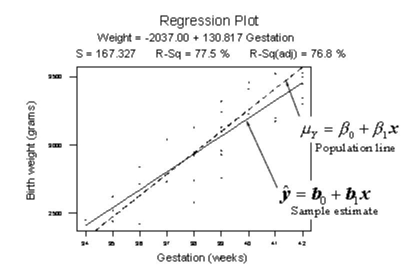
The dashed line summarizes the (unknown) relationship —\(\mu_Y = \beta_0+\beta_1x\)— between birth weight and gestation length of all births in the population. The solid line summarizes the relationship —\(\hat{y} = \beta_0+\beta_1x\)— between birth weight and gestation length in our random sample of 32 births. The goal of linear regression analysis is to use the solid line (the sample) in hopes of learning about the dashed line (the population).
Next... Confidence intervals and hypothesis tests
There are two ways to learn about a population parameter.
1) We can use confidence intervals to estimate parameters.
"We can be 95% confident that the proportion of Penn State students who have a tattoo is between 5.1% and 15.3%."
2) We can use hypothesis tests to test and ultimately draw conclusions about the value of a parameter.
"There is enough statistical evidence to conclude that the mean normal body temperature of adults is lower than 98.6 degrees F."
We review these two methods in the next two sections.
S.2 Confidence Intervals
S.2 Confidence IntervalsLet's review the basic concept of a confidence interval.
Suppose we want to estimate an actual population mean \(\mu\). As you know, we can only obtain \(\bar{x}\), the mean of a sample randomly selected from the population of interest. We can use \(\bar{x}\) to find a range of values:
\[\text{Lower value} < \text{population mean}\;\; \mu < \text{Upper value}\]
that we can be really confident contains the population mean \(\mu\). The range of values is called a "confidence interval."
Example S.2.1
Should using a hand-held cell phone while driving be illegal?
There is little doubt that you have seen numerous confidence intervals for population proportions reported in newspapers over the years.
For example, a newspaper report (ABC News poll, May 16-20, 2001) was concerned about whether or not U.S. adults thought using a hand-held cell phone while driving should be illegal. Of the 1,027 U.S. adults randomly selected for participation in the poll, 69% believed it should be illegal. The reporter claimed that the poll's "margin of error" was 3%. Therefore, the confidence interval for the (unknown) population proportion p is 69% ± 3%. That is, we can be really confident that between 66% and 72% of all U.S. adults think using a hand-held cell phone while driving a car should be illegal.
General Form of (Most) Confidence Intervals
The previous example illustrates the general form of most confidence intervals, namely:
$\text{Sample estimate} \pm \text{margin of error}$
The lower limit is obtained by:
$\text{the lower limit L of the interval} = \text{estimate} - \text{margin of error}$
The upper limit is obtained by:
$\text{the upper limit U of the interval} = \text{estimate} + \text{margin of error}$
Once we've obtained the interval, we can claim that we are really confident that the value of the population parameter is somewhere between the value of L and the value of U.
So far, we've been very general in our discussion of the calculation and interpretation of confidence intervals. To be more specific about their use, let's consider a specific interval, namely the "t-interval for a population mean µ."
(1-α)100% t-interval for the population mean \(\mu\)
If we are interested in estimating a population mean \(\mu\), it is very likely that we would use the t-interval for a population mean \(\mu\).
- t-Interval for a Population Mean
- The formula for the confidence interval in words is:
$\text{Sample mean} \pm (\text{t-multiplier} \times \text{standard error})$
- and you might recall that the formula for the confidence interval in notation is:
- $\bar{x}\pm t_{\alpha/2, n-1}\left(\dfrac{s}{\sqrt{n}}\right)$
Note that:
- the "t-multiplier," which we denote as \(t_{\alpha/2, n-1}\), depends on the sample size through n - 1 (called the "degrees of freedom") and the confidence level \((1-\alpha)\times100%\) through \(\frac{\alpha}{2}\).
- the "standard error," which is \(\frac{s}{\sqrt{n}}\), quantifies how much the sample means \(\bar{x}\) vary from sample to sample. That is, the standard error is just another name for the estimated standard deviation of all the possible sample means.
- the quantity to the right of the ± sign, i.e., "t-multiplier × standard error," is just a more specific form of the margin of error. That is, the margin of error in estimating a population mean µ is calculated by multiplying the t-multiplier by the standard error of the sample mean.
- the formula is only appropriate if a certain assumption is met, namely that the data are normally distributed.
Clearly, the sample mean \(\bar{x}\), the sample standard deviation s, and the sample size n are all readily obtained from the sample data. Now, we need to review how to obtain the value of the t-multiplier, and we'll be all set.
How is the t-multiplier determined?
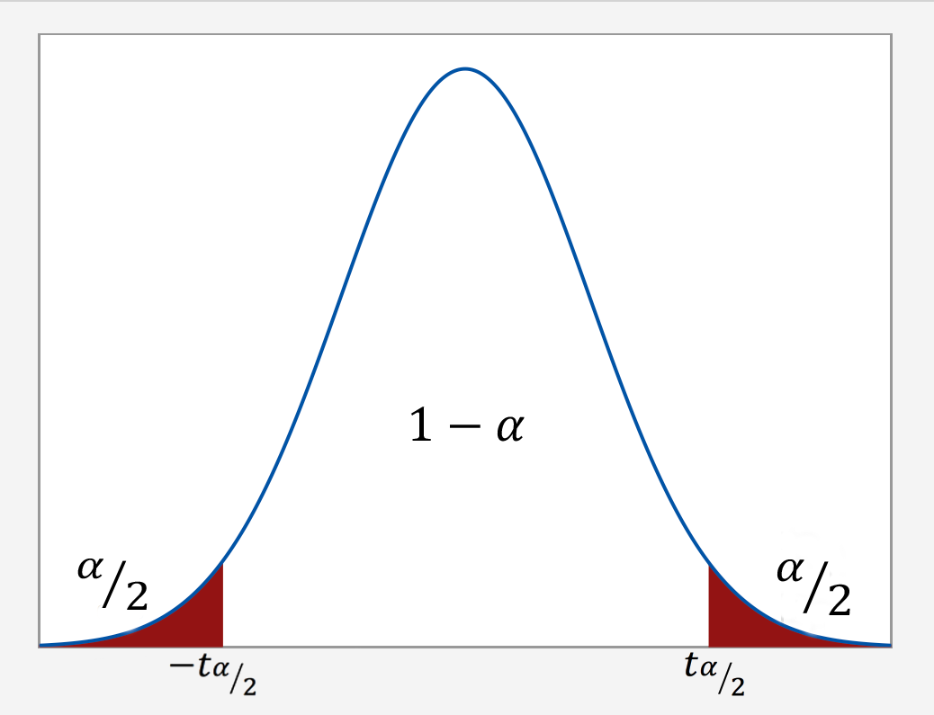
As the following graph illustrates, we put the confidence level $1-\alpha$ in the center of the t-distribution. Then, since the entire probability represented by the curve must equal 1, a probability of α must be shared equally among the two "tails" of the distribution. That is, the probability of the left tail is $\frac{\alpha}{2}$ and the probability of the right tail is $\frac{\alpha}{2}$. If we add up the probabilities of the various parts $(\frac{\alpha}{2} + 1-\alpha + \frac{\alpha}{2})$, we get 1. The t-multiplier, denoted \(t_{\alpha/2}\), is the t-value such that the probability "to the right of it" is $\frac{\alpha}{2}$:
It should be no surprise that we want to be as confident as possible when we estimate a population parameter. This is why confidence levels are typically very high. The most common confidence levels are 90%, 95%, and 99%. The following table contains a summary of the values of \(\frac{\alpha}{2}\) corresponding to these common confidence levels. (Note that the"confidence coefficient" is merely the confidence level reported as a proportion rather than as a percentage.)
| Confidence Coefficient $(1-\alpha)$ | Confidence Level $(1-\alpha) \times 100$ | $(1-\dfrac{\alpha}{2})$ | $\dfrac{\alpha}{2}$ |
|---|---|---|---|
| 0.90 | 90% | 0.95 | 0.05 |
| 0.95 | 95% | 0.975 | 0.025 |
| 0.99 | 99% | 0.995 | 0.005 |
Minitab® – Using Software
The good news is that statistical software, such as Minitab, will calculate most confidence intervals for us.
Let's take an example of researchers who are interested in the average heart rate of male college students. Assume a random sample of 130 male college students were taken for the study.
The following is the Minitab Output of a one-sample t-interval output using this data.
One-Sample T: Heart Rate
Descriptive Statistics
| N | Mean | StDev | SE Mean | 95% CI for $\mu$ |
|---|---|---|---|---|
| 130 | 73.762 | 7.062 | 0.619 | (72.536, 74.987) |
$\mu$: mean of HR
In this example, the researchers were interested in estimating \(\mu\), the heart rate. The output indicates that the mean for the sample of n = 130 male students equals 73.762. The sample standard deviation (StDev) is 7.062 and the estimated standard error of the mean (SE Mean) is 0.619. The 95% confidence interval for the population mean $\mu$ is (72.536, 74.987). We can be 95% confident that the mean heart rate of all male college students is between 72.536 and 74.987 beats per minute.
Factors Affecting the Width of the t-interval for the Mean $\mu$
Think about the width of the interval in the previous example. In general, do you think we desire narrow confidence intervals or wide confidence intervals? If you are not sure, consider the following two intervals:
- We are 95% confident that the average GPA of all college students is between 1.0 and 4.0.
- We are 95% confident that the average GPA of all college students is between 2.7 and 2.9.
Which of these two intervals is more informative? Of course, the narrower one gives us a better idea of the magnitude of the true unknown average GPA. In general, the narrower the confidence interval, the more information we have about the value of the population parameter. Therefore, we want all of our confidence intervals to be as narrow as possible. So, let's investigate what factors affect the width of the t-interval for the mean \(\mu\).
Of course, to find the width of the confidence interval, we just take the difference in the two limits:
Width = Upper Limit - Lower Limit
What factors affect the width of the confidence interval? We can examine this question by using the formula for the confidence interval and seeing what would happen should one of the elements of the formula be allowed to vary.
\[\bar{x}\pm t_{\alpha/2, n-1}\left(\dfrac{s}{\sqrt{n}}\right)\]
What is the width of the t-interval for the mean? If you subtract the lower limit from the upper limit, you get:
\[\text{Width }=2 \times t_{\alpha/2, n-1}\left(\dfrac{s}{\sqrt{n}}\right)\]
Now, let's investigate the factors that affect the length of this interval. Convince yourself that each of the following statements is accurate:
- As the sample mean increases, the length stays the same. That is, the sample mean plays no role in the width of the interval.
- As the sample standard deviation s decreases, the width of the interval decreases. Since s is an estimate of how much the data vary naturally, we have little control over s other than making sure that we make our measurements as carefully as possible.
- As we decrease the confidence level, the t-multiplier decreases, and hence the width of the interval decreases. In practice, we wouldn't want to set the confidence level below 90%.
- As we increase the sample size, the width of the interval decreases. This is the factor that we have the most flexibility in changing, the only limitation being our time and financial constraints.
In Closing
In our review of confidence intervals, we have focused on just one confidence interval. The important thing to recognize is that the topics discussed here — the general form of intervals, determination of t-multipliers, and factors affecting the width of an interval — generally extend to all of the confidence intervals we will encounter in this course.
S.3 Hypothesis Testing
S.3 Hypothesis TestingIn reviewing hypothesis tests, we start first with the general idea. Then, we keep returning to the basic procedures of hypothesis testing, each time adding a little more detail.
The general idea of hypothesis testing involves:
- Making an initial assumption.
- Collecting evidence (data).
- Based on the available evidence (data), deciding whether to reject or not reject the initial assumption.
Every hypothesis test — regardless of the population parameter involved — requires the above three steps.
Example S.3.1
Is Normal Body Temperature Really 98.6 Degrees F?
Consider the population of many, many adults. A researcher hypothesized that the average adult body temperature is lower than the often-advertised 98.6 degrees F. That is, the researcher wants an answer to the question: "Is the average adult body temperature 98.6 degrees? Or is it lower?" To answer his research question, the researcher starts by assuming that the average adult body temperature was 98.6 degrees F.
Then, the researcher went out and tried to find evidence that refutes his initial assumption. In doing so, he selects a random sample of 130 adults. The average body temperature of the 130 sampled adults is 98.25 degrees.
Then, the researcher uses the data he collected to make a decision about his initial assumption. It is either likely or unlikely that the researcher would collect the evidence he did given his initial assumption that the average adult body temperature is 98.6 degrees:
- If it is likely, then the researcher does not reject his initial assumption that the average adult body temperature is 98.6 degrees. There is not enough evidence to do otherwise.
- If it is unlikely, then:
- either the researcher's initial assumption is correct and he experienced a very unusual event;
- or the researcher's initial assumption is incorrect.
In statistics, we generally don't make claims that require us to believe that a very unusual event happened. That is, in the practice of statistics, if the evidence (data) we collected is unlikely in light of the initial assumption, then we reject our initial assumption.
Example S.3.2
Criminal Trial Analogy
One place where you can consistently see the general idea of hypothesis testing in action is in criminal trials held in the United States. Our criminal justice system assumes "the defendant is innocent until proven guilty." That is, our initial assumption is that the defendant is innocent.
In the practice of statistics, we make our initial assumption when we state our two competing hypotheses -- the null hypothesis (H0) and the alternative hypothesis (HA). Here, our hypotheses are:
- H0: Defendant is not guilty (innocent)
- HA: Defendant is guilty
In statistics, we always assume the null hypothesis is true. That is, the null hypothesis is always our initial assumption.
The prosecution team then collects evidence — such as finger prints, blood spots, hair samples, carpet fibers, shoe prints, ransom notes, and handwriting samples — with the hopes of finding "sufficient evidence" to make the assumption of innocence refutable.
In statistics, the data are the evidence.
The jury then makes a decision based on the available evidence:
- If the jury finds sufficient evidence — beyond a reasonable doubt — to make the assumption of innocence refutable, the jury rejects the null hypothesis and deems the defendant guilty. We behave as if the defendant is guilty.
- If there is insufficient evidence, then the jury does not reject the null hypothesis. We behave as if the defendant is innocent.
In statistics, we always make one of two decisions. We either "reject the null hypothesis" or we "fail to reject the null hypothesis."
Errors in Hypothesis Testing
Did you notice the use of the phrase "behave as if" in the previous discussion? We "behave as if" the defendant is guilty; we do not "prove" that the defendant is guilty. And, we "behave as if" the defendant is innocent; we do not "prove" that the defendant is innocent.
This is a very important distinction! We make our decision based on evidence not on 100% guaranteed proof. Again:
- If we reject the null hypothesis, we do not prove that the alternative hypothesis is true.
- If we do not reject the null hypothesis, we do not prove that the null hypothesis is true.
We merely state that there is enough evidence to behave one way or the other. This is always true in statistics! Because of this, whatever the decision, there is always a chance that we made an error.
Let's review the two types of errors that can be made in criminal trials:
| Jury Decision | Truth | ||
|---|---|---|---|
| Not Guilty | Guilty | ||
| Not Guilty | OK | ERROR | |
| Guilty | ERROR | OK | |
Table S.3.2 shows how this corresponds to the two types of errors in hypothesis testing.
| Decision | Truth | ||
|---|---|---|---|
| Null Hypothesis | Alternative Hypothesis | ||
| Do not Reject Null | OK | Type II Error | |
| Reject Null | Type I Error | OK | |
Note that, in statistics, we call the two types of errors by two different names -- one is called a "Type I error," and the other is called a "Type II error." Here are the formal definitions of the two types of errors:
- Type I Error
- The null hypothesis is rejected when it is true.
- Type II Error
- The null hypothesis is not rejected when it is false.
There is always a chance of making one of these errors. But, a good scientific study will minimize the chance of doing so!
Making the Decision
Recall that it is either likely or unlikely that we would observe the evidence we did given our initial assumption. If it is likely, we do not reject the null hypothesis. If it is unlikely, then we reject the null hypothesis in favor of the alternative hypothesis. Effectively, then, making the decision reduces to determining "likely" or "unlikely."
In statistics, there are two ways to determine whether the evidence is likely or unlikely given the initial assumption:
- We could take the "critical value approach" (favored in many of the older textbooks).
- Or, we could take the "P-value approach" (what is used most often in research, journal articles, and statistical software).
In the next two sections, we review the procedures behind each of these two approaches. To make our review concrete, let's imagine that μ is the average grade point average of all American students who major in mathematics. We first review the critical value approach for conducting each of the following three hypothesis tests about the population mean $\mu$:
|
Type
|
Null
|
Alternative
|
|---|---|---|
|
Right-tailed
|
H0 : μ = 3
|
HA : μ > 3
|
|
Left-tailed
|
H0 : μ = 3
|
HA : μ < 3
|
|
Two-tailed
|
H0 : μ = 3
|
HA : μ ≠ 3
|
In Practice
-
We would want to conduct the first hypothesis test if we were interested in concluding that the average grade point average of the group is more than 3.
-
We would want to conduct the second hypothesis test if we were interested in concluding that the average grade point average of the group is less than 3.
-
And, we would want to conduct the third hypothesis test if we were only interested in concluding that the average grade point average of the group differs from 3 (without caring whether it is more or less than 3).
Upon completing the review of the critical value approach, we review the P-value approach for conducting each of the above three hypothesis tests about the population mean \(\mu\). The procedures that we review here for both approaches easily extend to hypothesis tests about any other population parameter.
S.3.1 Hypothesis Testing (Critical Value Approach)
S.3.1 Hypothesis Testing (Critical Value Approach)The critical value approach involves determining "likely" or "unlikely" by determining whether or not the observed test statistic is more extreme than would be expected if the null hypothesis were true. That is, it entails comparing the observed test statistic to some cutoff value, called the "critical value." If the test statistic is more extreme than the critical value, then the null hypothesis is rejected in favor of the alternative hypothesis. If the test statistic is not as extreme as the critical value, then the null hypothesis is not rejected.
Specifically, the four steps involved in using the critical value approach to conducting any hypothesis test are:
- Specify the null and alternative hypotheses.
- Using the sample data and assuming the null hypothesis is true, calculate the value of the test statistic. To conduct the hypothesis test for the population mean μ, we use the t-statistic \(t^*=\frac{\bar{x}-\mu}{s/\sqrt{n}}\) which follows a t-distribution with n - 1 degrees of freedom.
- Determine the critical value by finding the value of the known distribution of the test statistic such that the probability of making a Type I error — which is denoted \(\alpha\) (greek letter "alpha") and is called the "significance level of the test" — is small (typically 0.01, 0.05, or 0.10).
- Compare the test statistic to the critical value. If the test statistic is more extreme in the direction of the alternative than the critical value, reject the null hypothesis in favor of the alternative hypothesis. If the test statistic is less extreme than the critical value, do not reject the null hypothesis.
Example S.3.1.1
Mean GPA
In our example concerning the mean grade point average, suppose we take a random sample of n = 15 students majoring in mathematics. Since n = 15, our test statistic t* has n - 1 = 14 degrees of freedom. Also, suppose we set our significance level α at 0.05 so that we have only a 5% chance of making a Type I error.
Right-Tailed
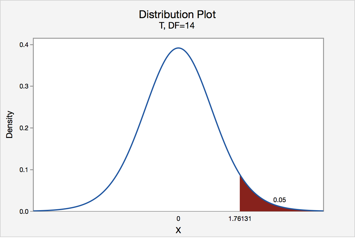
The critical value for conducting the right-tailed test H0 : μ = 3 versus HA : μ > 3 is the t-value, denoted t\(\alpha\), n - 1, such that the probability to the right of it is \(\alpha\). It can be shown using either statistical software or a t-table that the critical value t 0.05,14 is 1.7613. That is, we would reject the null hypothesis H0 : μ = 3 in favor of the alternative hypothesis HA : μ > 3 if the test statistic t* is greater than 1.7613. Visually, the rejection region is shaded red in the graph.
Left-Tailed
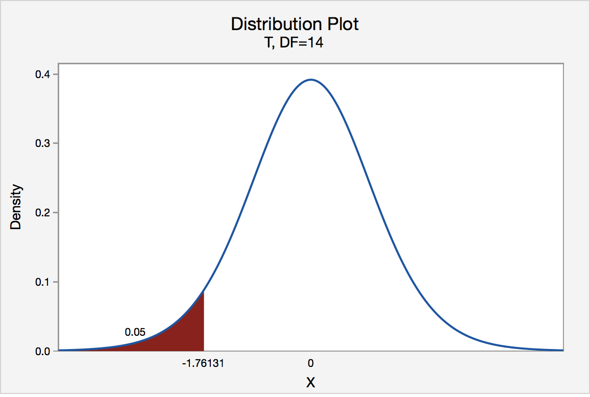
The critical value for conducting the left-tailed test H0 : μ = 3 versus HA : μ < 3 is the t-value, denoted -t(\(\alpha\), n - 1), such that the probability to the left of it is \(\alpha\). It can be shown using either statistical software or a t-table that the critical value -t0.05,14 is -1.7613. That is, we would reject the null hypothesis H0 : μ = 3 in favor of the alternative hypothesis HA : μ < 3 if the test statistic t* is less than -1.7613. Visually, the rejection region is shaded red in the graph.
Two-Tailed
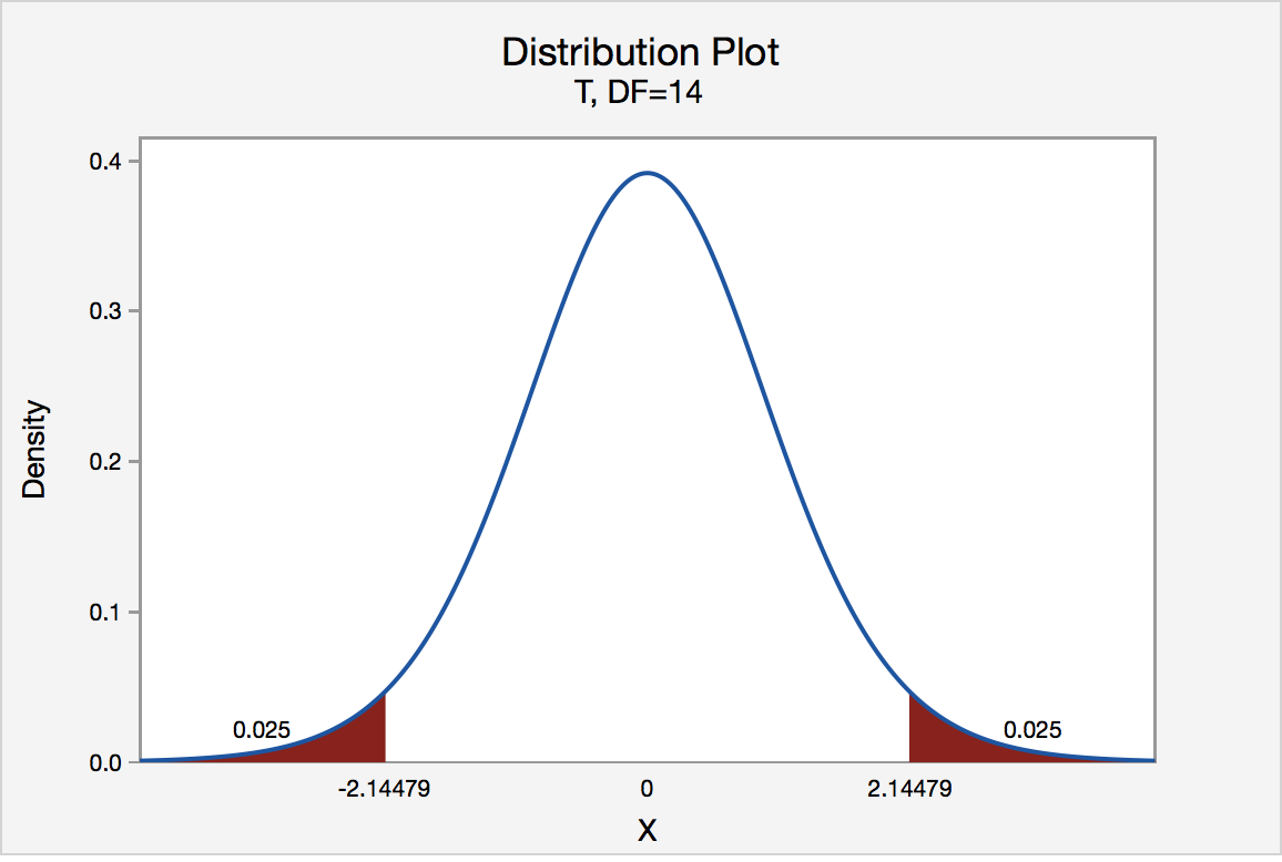
There are two critical values for the two-tailed test H0 : μ = 3 versus HA : μ ≠ 3 — one for the left-tail denoted -t(\(\alpha\)/2, n - 1) and one for the right-tail denoted t(\(\alpha\)/2, n - 1). The value -t(\(\alpha\)/2, n - 1) is the t-value such that the probability to the left of it is \(\alpha\)/2, and the value t(\(\alpha\)/2, n - 1) is the t-value such that the probability to the right of it is \(\alpha\)/2. It can be shown using either statistical software or a t-table that the critical value -t0.025,14 is -2.1448 and the critical value t0.025,14 is 2.1448. That is, we would reject the null hypothesis H0 : μ = 3 in favor of the alternative hypothesis HA : μ ≠ 3 if the test statistic t* is less than -2.1448 or greater than 2.1448. Visually, the rejection region is shaded red in the graph.
S.3.2 Hypothesis Testing (P-Value Approach)
S.3.2 Hypothesis Testing (P-Value Approach)The P-value approach involves determining "likely" or "unlikely" by determining the probability — assuming the null hypothesis was true — of observing a more extreme test statistic in the direction of the alternative hypothesis than the one observed. If the P-value is small, say less than (or equal to) \(\alpha\), then it is "unlikely." And, if the P-value is large, say more than \(\alpha\), then it is "likely."
If the P-value is less than (or equal to) \(\alpha\), then the null hypothesis is rejected in favor of the alternative hypothesis. And, if the P-value is greater than \(\alpha\), then the null hypothesis is not rejected.
Specifically, the four steps involved in using the P-value approach to conducting any hypothesis test are:
- Specify the null and alternative hypotheses.
- Using the sample data and assuming the null hypothesis is true, calculate the value of the test statistic. Again, to conduct the hypothesis test for the population mean μ, we use the t-statistic \(t^*=\frac{\bar{x}-\mu}{s/\sqrt{n}}\) which follows a t-distribution with n - 1 degrees of freedom.
- Using the known distribution of the test statistic, calculate the P-value: "If the null hypothesis is true, what is the probability that we'd observe a more extreme test statistic in the direction of the alternative hypothesis than we did?" (Note how this question is equivalent to the question answered in criminal trials: "If the defendant is innocent, what is the chance that we'd observe such extreme criminal evidence?")
- Set the significance level, \(\alpha\), the probability of making a Type I error to be small — 0.01, 0.05, or 0.10. Compare the P-value to \(\alpha\). If the P-value is less than (or equal to) \(\alpha\), reject the null hypothesis in favor of the alternative hypothesis. If the P-value is greater than \(\alpha\), do not reject the null hypothesis.
Example S.3.2.1
Mean GPA
In our example concerning the mean grade point average, suppose that our random sample of n = 15 students majoring in mathematics yields a test statistic t* equaling 2.5. Since n = 15, our test statistic t* has n - 1 = 14 degrees of freedom. Also, suppose we set our significance level α at 0.05 so that we have only a 5% chance of making a Type I error.
Right Tailed
The P-value for conducting the right-tailed test H0 : μ = 3 versus HA : μ > 3 is the probability that we would observe a test statistic greater than t* = 2.5 if the population mean \(\mu\) really were 3. Recall that probability equals the area under the probability curve. The P-value is therefore the area under a tn - 1 = t14 curve and to the right of the test statistic t* = 2.5. It can be shown using statistical software that the P-value is 0.0127. The graph depicts this visually.
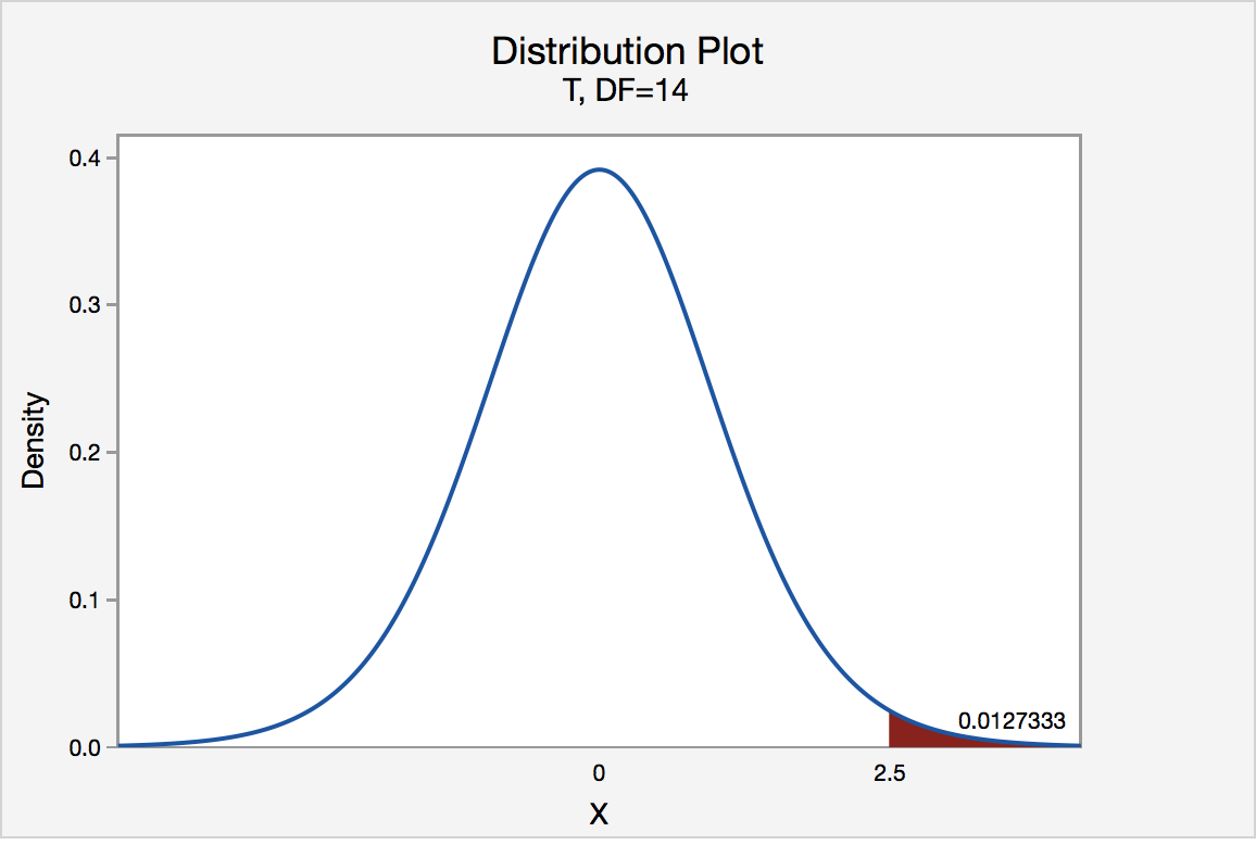
The P-value, 0.0127, tells us it is "unlikely" that we would observe such an extreme test statistic t* in the direction of HA if the null hypothesis were true. Therefore, our initial assumption that the null hypothesis is true must be incorrect. That is, since the P-value, 0.0127, is less than \(\alpha\) = 0.05, we reject the null hypothesis H0 : μ = 3 in favor of the alternative hypothesis HA : μ > 3.
Note that we would not reject H0 : μ = 3 in favor of HA : μ > 3 if we lowered our willingness to make a Type I error to \(\alpha\) = 0.01 instead, as the P-value, 0.0127, is then greater than \(\alpha\) = 0.01.
Left Tailed
In our example concerning the mean grade point average, suppose that our random sample of n = 15 students majoring in mathematics yields a test statistic t* instead of equaling -2.5. The P-value for conducting the left-tailed test H0 : μ = 3 versus HA : μ < 3 is the probability that we would observe a test statistic less than t* = -2.5 if the population mean μ really were 3. The P-value is therefore the area under a tn - 1 = t14 curve and to the left of the test statistic t* = -2.5. It can be shown using statistical software that the P-value is 0.0127. The graph depicts this visually.
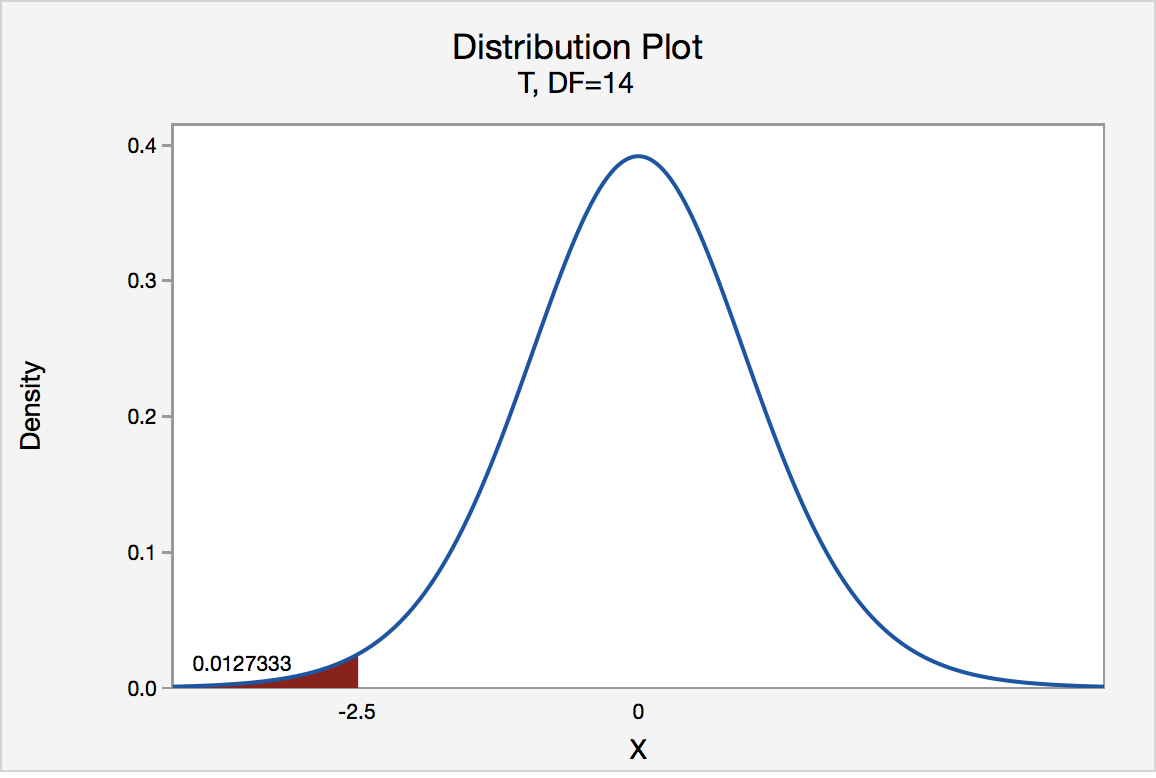
The P-value, 0.0127, tells us it is "unlikely" that we would observe such an extreme test statistic t* in the direction of HA if the null hypothesis were true. Therefore, our initial assumption that the null hypothesis is true must be incorrect. That is, since the P-value, 0.0127, is less than α = 0.05, we reject the null hypothesis H0 : μ = 3 in favor of the alternative hypothesis HA : μ < 3.
Note that we would not reject H0 : μ = 3 in favor of HA : μ < 3 if we lowered our willingness to make a Type I error to α = 0.01 instead, as the P-value, 0.0127, is then greater than \(\alpha\) = 0.01.
Two-Tailed
In our example concerning the mean grade point average, suppose again that our random sample of n = 15 students majoring in mathematics yields a test statistic t* instead of equaling -2.5. The P-value for conducting the two-tailed test H0 : μ = 3 versus HA : μ ≠ 3 is the probability that we would observe a test statistic less than -2.5 or greater than 2.5 if the population mean μ really was 3. That is, the two-tailed test requires taking into account the possibility that the test statistic could fall into either tail (hence the name "two-tailed" test). The P-value is, therefore, the area under a tn - 1 = t14 curve to the left of -2.5 and to the right of 2.5. It can be shown using statistical software that the P-value is 0.0127 + 0.0127, or 0.0254. The graph depicts this visually.
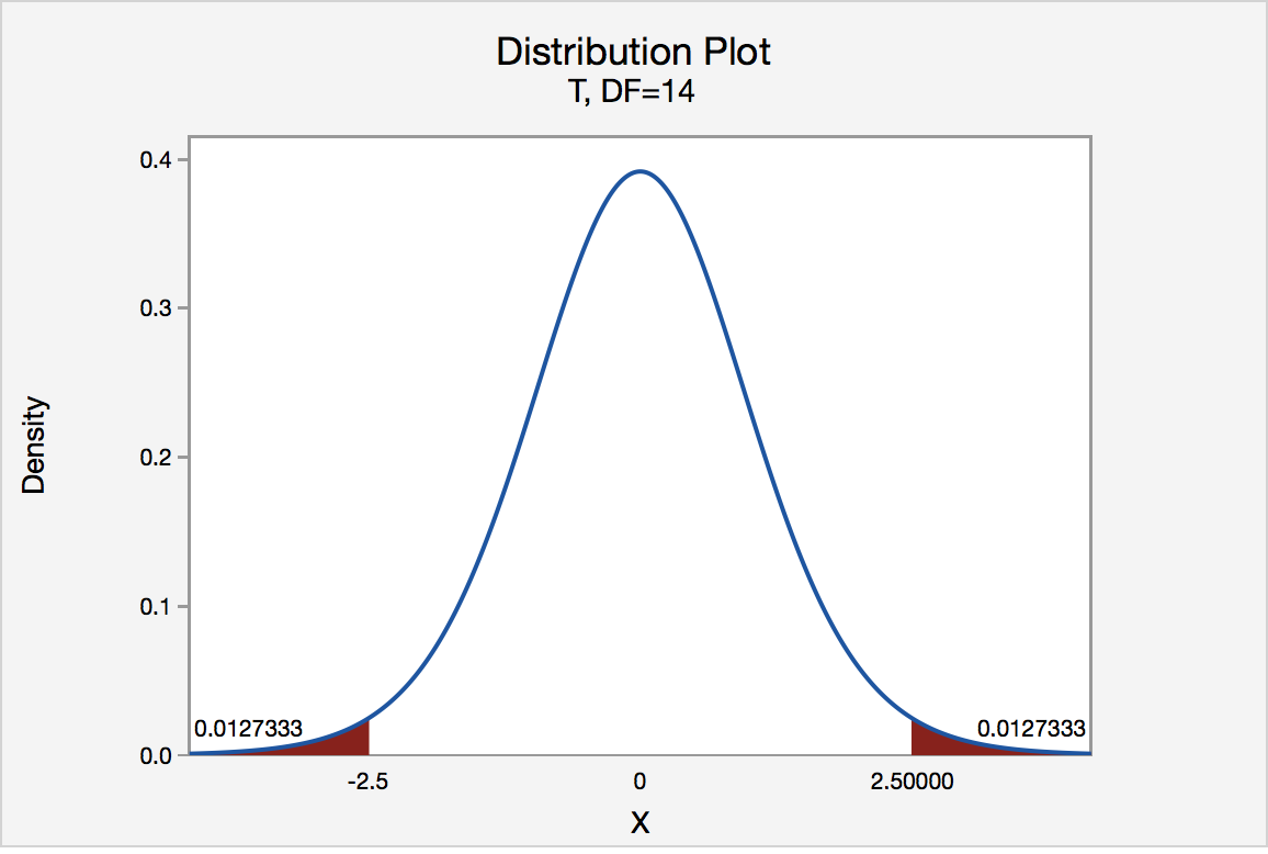
Note that the P-value for a two-tailed test is always two times the P-value for either of the one-tailed tests. The P-value, 0.0254, tells us it is "unlikely" that we would observe such an extreme test statistic t* in the direction of HA if the null hypothesis were true. Therefore, our initial assumption that the null hypothesis is true must be incorrect. That is, since the P-value, 0.0254, is less than α = 0.05, we reject the null hypothesis H0 : μ = 3 in favor of the alternative hypothesis HA : μ ≠ 3.
Note that we would not reject H0 : μ = 3 in favor of HA : μ ≠ 3 if we lowered our willingness to make a Type I error to α = 0.01 instead, as the P-value, 0.0254, is then greater than \(\alpha\) = 0.01.
Now that we have reviewed the critical value and P-value approach procedures for each of the three possible hypotheses, let's look at three new examples — one of a right-tailed test, one of a left-tailed test, and one of a two-tailed test.
The good news is that, whenever possible, we will take advantage of the test statistics and P-values reported in statistical software, such as Minitab, to conduct our hypothesis tests in this course.
S.3.3 Hypothesis Testing Examples
S.3.3 Hypothesis Testing ExamplesBrinell Hardness Scores
An engineer measured the Brinell hardness of 25 pieces of ductile iron that were subcritically annealed. The resulting data were:
| Brinell Hardness of 25 Pieces of Ductile Iron | ||||||||
|---|---|---|---|---|---|---|---|---|
| 170 | 167 | 174 | 179 | 179 | 187 | 179 | 183 | 179 |
| 156 | 163 | 156 | 187 | 156 | 167 | 156 | 174 | 170 |
| 183 | 179 | 174 | 179 | 170 | 159 | 187 | ||
The engineer hypothesized that the mean Brinell hardness of all such ductile iron pieces is greater than 170. Therefore, he was interested in testing the hypotheses:
H0 : μ = 170
HA : μ > 170
The engineer entered his data into Minitab and requested that the "one-sample t-test" be conducted for the above hypotheses. He obtained the following output:
Descriptive Statistics
| N | Mean | StDev | SE Mean | 95% Lower Bound |
|---|---|---|---|---|
| 25 | 172.52 | 10.31 | 2.06 | 168.99 |
$\mu$: mean of Brinelli
Test
Null hypothesis H₀: $\mu$ = 170
Alternative hypothesis H₁: $\mu$ > 170
| T-Value | P-Value |
|---|---|
| 1.22 | 0.117 |
The output tells us that the average Brinell hardness of the n = 25 pieces of ductile iron was 172.52 with a standard deviation of 10.31. (The standard error of the mean "SE Mean", calculated by dividing the standard deviation 10.31 by the square root of n = 25, is 2.06). The test statistic t* is 1.22, and the P-value is 0.117.
If the engineer set his significance level α at 0.05 and used the critical value approach to conduct his hypothesis test, he would reject the null hypothesis if his test statistic t* were greater than 1.7109 (determined using statistical software or a t-table):
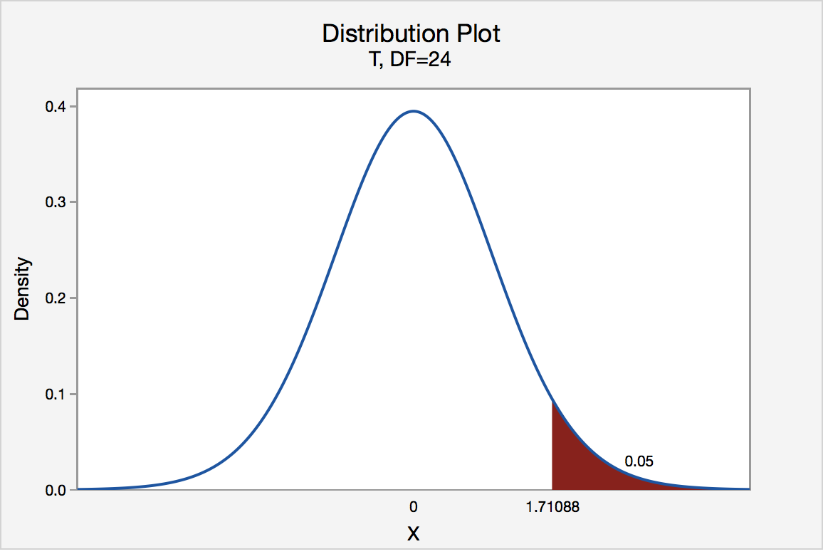
Since the engineer's test statistic, t* = 1.22, is not greater than 1.7109, the engineer fails to reject the null hypothesis. That is, the test statistic does not fall in the "critical region." There is insufficient evidence, at the \(\alpha\) = 0.05 level, to conclude that the mean Brinell hardness of all such ductile iron pieces is greater than 170.
If the engineer used the P-value approach to conduct his hypothesis test, he would determine the area under a tn - 1 = t24 curve and to the right of the test statistic t* = 1.22:
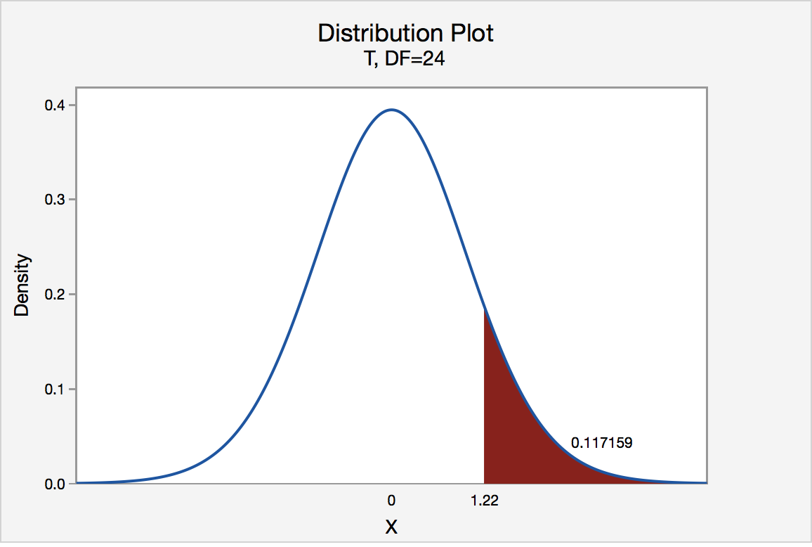
In the output above, Minitab reports that the P-value is 0.117. Since the P-value, 0.117, is greater than \(\alpha\) = 0.05, the engineer fails to reject the null hypothesis. There is insufficient evidence, at the \(\alpha\) = 0.05 level, to conclude that the mean Brinell hardness of all such ductile iron pieces is greater than 170.
Note that the engineer obtains the same scientific conclusion regardless of the approach used. This will always be the case.
Height of Sunflowers
A biologist was interested in determining whether sunflower seedlings treated with an extract from Vinca minor roots resulted in a lower average height of sunflower seedlings than the standard height of 15.7 cm. The biologist treated a random sample of n = 33 seedlings with the extract and subsequently obtained the following heights:
| Heights of 33 Sunflower Seedlings | ||||||||
|---|---|---|---|---|---|---|---|---|
| 11.5 | 11.8 | 15.7 | 16.1 | 14.1 | 10.5 | 9.3 | 15.0 | 11.1 |
| 15.2 | 19.0 | 12.8 | 12.4 | 19.2 | 13.5 | 12.2 | 13.3 | |
| 16.5 | 13.5 | 14.4 | 16.7 | 10.9 | 13.0 | 10.3 | 15.8 | |
| 15.1 | 17.1 | 13.3 | 12.4 | 8.5 | 14.3 | 12.9 | 13.5 | |
The biologist's hypotheses are:
H0 : μ = 15.7
HA : μ < 15.7
The biologist entered her data into Minitab and requested that the "one-sample t-test" be conducted for the above hypotheses. She obtained the following output:
Descriptive Statistics
| N | Mean | StDev | SE Mean | 95% Upper Bound |
|---|---|---|---|---|
| 33 | 13.664 | 2.544 | 0.443 | 14.414 |
$\mu$: mean of Height
Test
Null hypothesis H₀: $\mu$ = 15.7
Alternative hypothesis H₁: $\mu$ < 15.7
| T-Value | P-Value |
|---|---|
| -4.60 | 0.000 |
The output tells us that the average height of the n = 33 sunflower seedlings was 13.664 with a standard deviation of 2.544. (The standard error of the mean "SE Mean", calculated by dividing the standard deviation 13.664 by the square root of n = 33, is 0.443). The test statistic t* is -4.60, and the P-value, 0.000, is to three decimal places.
Minitab Note. Minitab will always report P-values to only 3 decimal places. If Minitab reports the P-value as 0.000, it really means that the P-value is 0.000....something. Throughout this course (and your future research!), when you see that Minitab reports the P-value as 0.000, you should report the P-value as being "< 0.001."
If the biologist set her significance level \(\alpha\) at 0.05 and used the critical value approach to conduct her hypothesis test, she would reject the null hypothesis if her test statistic t* were less than -1.6939 (determined using statistical software or a t-table):s-3-3
Since the biologist's test statistic, t* = -4.60, is less than -1.6939, the biologist rejects the null hypothesis. That is, the test statistic falls in the "critical region." There is sufficient evidence, at the α = 0.05 level, to conclude that the mean height of all such sunflower seedlings is less than 15.7 cm.
If the biologist used the P-value approach to conduct her hypothesis test, she would determine the area under a tn - 1 = t32 curve and to the left of the test statistic t* = -4.60:
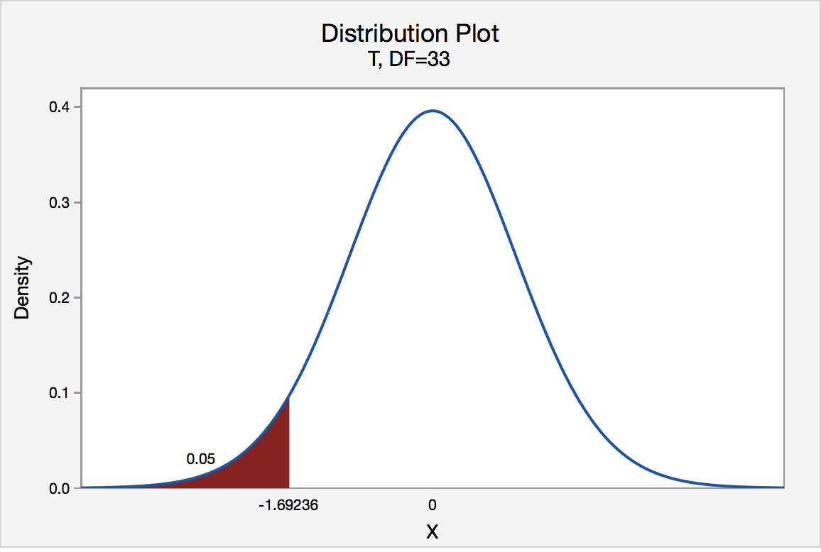
In the output above, Minitab reports that the P-value is 0.000, which we take to mean < 0.001. Since the P-value is less than 0.001, it is clearly less than \(\alpha\) = 0.05, and the biologist rejects the null hypothesis. There is sufficient evidence, at the \(\alpha\) = 0.05 level, to conclude that the mean height of all such sunflower seedlings is less than 15.7 cm.
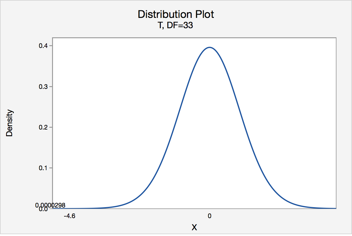
Note again that the biologist obtains the same scientific conclusion regardless of the approach used. This will always be the case.
Gum Thickness
A manufacturer claims that the thickness of the spearmint gum it produces is 7.5 one-hundredths of an inch. A quality control specialist regularly checks this claim. On one production run, he took a random sample of n = 10 pieces of gum and measured their thickness. He obtained:
| Thicknesses of 10 Pieces of Gum | ||||
|---|---|---|---|---|
| 7.65 | 7.60 | 7.65 | 7.70 | 7.55 |
| 7.55 | 7.40 | 7.40 | 7.50 | 7.50 |
The quality control specialist's hypotheses are:
H0 : μ = 7.5
HA : μ ≠ 7.5
The quality control specialist entered his data into Minitab and requested that the "one-sample t-test" be conducted for the above hypotheses. He obtained the following output:
Descriptive Statistics
| N | Mean | StDev | SE Mean | 95% CI for $\mu$ |
|---|---|---|---|---|
| 10 | 7.550 | 0.1027 | 0.0325 | (7.4765, 7.6235) |
$\mu$: mean of Thickness
Test
Null hypothesis H₀: $\mu$ = 7.5
Alternative hypothesis H₁: $\mu \ne$ 7.5
| T-Value | P-Value |
|---|---|
| 1.54 | 0.158 |
The output tells us that the average thickness of the n = 10 pieces of gums was 7.55 one-hundredths of an inch with a standard deviation of 0.1027. (The standard error of the mean "SE Mean", calculated by dividing the standard deviation 0.1027 by the square root of n = 10, is 0.0325). The test statistic t* is 1.54, and the P-value is 0.158.
If the quality control specialist sets his significance level \(\alpha\) at 0.05 and used the critical value approach to conduct his hypothesis test, he would reject the null hypothesis if his test statistic t* were less than -2.2616 or greater than 2.2616 (determined using statistical software or a t-table):
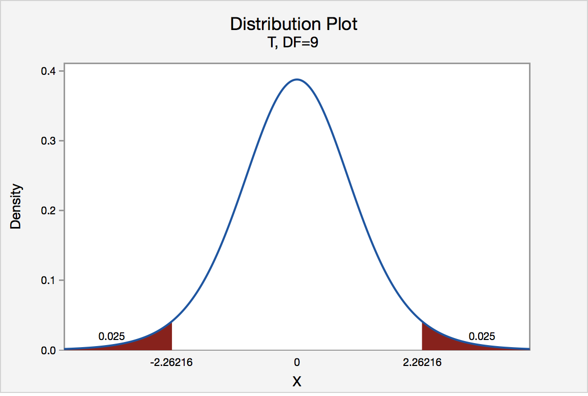
Since the quality control specialist's test statistic, t* = 1.54, is not less than -2.2616 nor greater than 2.2616, the quality control specialist fails to reject the null hypothesis. That is, the test statistic does not fall in the "critical region." There is insufficient evidence, at the \(\alpha\) = 0.05 level, to conclude that the mean thickness of all of the manufacturer's spearmint gum differs from 7.5 one-hundredths of an inch.
If the quality control specialist used the P-value approach to conduct his hypothesis test, he would determine the area under a tn - 1 = t9 curve, to the right of 1.54 and to the left of -1.54:
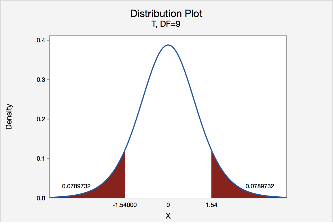
In the output above, Minitab reports that the P-value is 0.158. Since the P-value, 0.158, is greater than \(\alpha\) = 0.05, the quality control specialist fails to reject the null hypothesis. There is insufficient evidence, at the \(\alpha\) = 0.05 level, to conclude that the mean thickness of all pieces of spearmint gum differs from 7.5 one-hundredths of an inch.
Note that the quality control specialist obtains the same scientific conclusion regardless of the approach used. This will always be the case.
In closing
In our review of hypothesis tests, we have focused on just one particular hypothesis test, namely that concerning the population mean \(\mu\). The important thing to recognize is that the topics discussed here — the general idea of hypothesis tests, errors in hypothesis testing, the critical value approach, and the P-value approach — generally extend to all of the hypothesis tests you will encounter.
S.4 Chi-Square Tests
S.4 Chi-Square TestsChi-Square Test of Independence
Do you remember how to test the independence of two categorical variables? This test is performed by using a Chi-square test of independence.
Recall that we can summarize two categorical variables within a two-way table, also called an r × c contingency table, where r = number of rows, c = number of columns. Our question of interest is “Are the two variables independent?” This question is set up using the following hypothesis statements:
- Null Hypothesis
- The two categorical variables are independent
- Alternative Hypothesis
- The two categorical variables are dependent
- Chi-Square Test Statistic
- \(\chi^2=\sum(O-E)^2/E\)
- where O represents the observed frequency. E is the expected frequency under the null hypothesis and computed by:
\[E=\frac{\text{row total}\times\text{column total}}{\text{sample size}}\]
We will compare the value of the test statistic to the critical value of \(\chi_{\alpha}^2\) with the degree of freedom = (r - 1) (c - 1), and reject the null hypothesis if \(\chi^2 \gt \chi_{\alpha}^2\).
Example S.4.1
Is gender independent of education level? A random sample of 395 people was surveyed and each person was asked to report the highest education level they obtained. The data that resulted from the survey are summarized in the following table:
| High School | Bachelors | Masters | Ph.d. | Total | |
|---|---|---|---|---|---|
| Female | 60 | 54 | 46 | 41 | 201 |
| Male | 40 | 44 | 53 | 57 | 194 |
| Total | 100 | 98 | 99 | 98 | 395 |
Question: Are gender and education level dependent at a 5% level of significance? In other words, given the data collected above, is there a relationship between the gender of an individual and the level of education that they have obtained?
Here's the table of expected counts:
| High School | Bachelors | Masters | Ph.d. | Total | |
|---|---|---|---|---|---|
| Female | 50.886 | 49.868 | 50.377 | 49.868 | 201 |
| Male | 49.114 | 48.132 | 48.623 | 48.132 | 194 |
| Total | 100 | 98 | 99 | 98 | 395 |
So, working this out, \(\chi^2= \dfrac{(60−50.886)^2}{50.886} + \cdots + \dfrac{(57 − 48.132)^2}{48.132} = 8.006\)
The critical value of \(\chi^2\) with 3 degrees of freedom is 7.815. Since 8.006 > 7.815, we reject the null hypothesis and conclude that the education level depends on gender at a 5% level of significance.
S.5 Power Analysis
S.5 Power AnalysisWhy is Power Analysis Important?
Consider a research experiment where the p-value computed from the data was 0.12. As a result, one would fail to reject the null hypothesis because this p-value is larger than \(\alpha\) = 0.05. However, there still exist two possible cases for which we failed to reject the null hypothesis:
- the null hypothesis is a reasonable conclusion,
- the sample size is not large enough to either accept or reject the null hypothesis, i.e., additional samples might provide additional evidence.
Power analysis is the procedure that researchers can use to determine if the test contains enough power to make a reasonable conclusion. From another perspective power analysis can also be used to calculate the number of samples required to achieve a specified level of power.
Example S.5.1
Let's take a look at an example that illustrates how to compute the power of the test.
Example
Let X denote the height of randomly selected Penn State students. Assume that X is normally distributed with unknown mean \(\mu\) and a standard deviation of 9. Take a random sample of n = 25 students, so that, after setting the probability of committing a Type I error at \(\alpha = 0.05\), we can test the null hypothesis \(H_0: \mu = 170\) against the alternative hypothesis that \(H_A: \mu > 170\).
What is the power of the hypothesis test if the true population mean were \(\mu = 175\)?
\[\begin{align}z&=\frac{\bar{x}-\mu}{\sigma / \sqrt{n}} \\
\bar{x}&= \mu + z \left(\frac{\sigma}{\sqrt{n}}\right) \\
\bar{x}&=170+1.645\left(\frac{9}{\sqrt{25}}\right) \\
&=172.961\\
\end{align}\]
So we should reject the null hypothesis when the observed sample mean is 172.961 or greater:
We get
\[\begin{align}\text{Power}&=P(\bar{x} \ge 172.961 \text{ when } \mu =175)\\
&=P\left(z \ge \frac{172.961-175}{9/\sqrt{25}} \right)\\
&=P(z \ge -1.133)\\
&= 0.8713\\
\end{align}\]
and illustrated below:
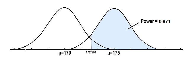
In summary, we have determined that we have an 87.13% chance of rejecting the null hypothesis \(H_0: \mu = 170\) in favor of the alternative hypothesis \(H_A: \mu > 170\) if the true unknown population mean is, in reality, \(\mu = 175\).
Calculating Sample Size
If the sample size is fixed, then decreasing Type I error \(\alpha\) will increase Type II error \(\beta\). If one wants both to decrease, then one has to increase the sample size.
To calculate the smallest sample size needed for specified \(\alpha\), \(\beta\), \(\mu_a\), then (\(\mu_a\) is the likely value of \(\mu\) at which you want to evaluate the power.
- Sample Size for One-Tailed Test
- \(n = \dfrac{\sigma^2(Z_{\alpha}+Z_{\beta})^2}{(\mu_0−\mu_a)^2}\)
- Sample Size for Two-Tailed Test
- \(n = \dfrac{\sigma^2(Z_{\alpha/2}+Z_{\beta})^2}{(\mu_0−\mu_a)^2}\)
Let's investigate by returning to our previous example.
Example S.5.2
Let X denote the height of randomly selected Penn State students. Assume that X is normally distributed with unknown mean \(\mu\) and standard deviation 9. We are interested in testing at \(\alpha = 0.05\) level , the null hypothesis \(H_0: \mu = 170\) against the alternative hypothesis that \(H_A: \mu > 170\).
Find the sample size n that is necessary to achieve 0.90 power at the alternative μ = 175.
\[\begin{align}n&= \dfrac{\sigma^2(Z_{\alpha}+Z_{\beta})^2}{(\mu_0−\mu_a)^2}\\ &=\dfrac{9^2 (1.645 + 1.28)^2}{(170-175)^2}\\ &=27.72\\ n&=28\\ \end{align}\]
In summary, you should see how power analysis is very important so that we are able to make the correct decision when the data indicate that one cannot reject the null hypothesis. You should also see how power analysis can also be used to calculate the minimum sample size required to detect a difference that meets the needs of your research.
S.6 Test of Proportion
S.6 Test of ProportionLet us consider the parameter p of the population proportion. For instance, we might want to know the proportion of males within a total population of adults when we conduct a survey. A test of proportion will assess whether or not a sample from a population represents the true proportion of the entire population.
Critical Value Approach
The steps to perform a test of proportion using the critical value approval are as follows:
- State the null hypothesis H0 and the alternative hypothesis HA.
- Calculate the test statistic:
\[z=\frac{\hat{p}-p_0}{\sqrt{\frac{p_0(1-p_0)}{n}}}\]
where \(p_0\) is the null hypothesized proportion i.e., when \(H_0: p=p_0\)
-
Determine the critical region.
-
Make a decision. Determine if the test statistic falls in the critical region. If it does, reject the null hypothesis. If it does not, do not reject the null hypothesis.
Example S.6.1
Newborn babies are more likely to be boys than girls. A random sample found 13,173 boys were born among 25,468 newborn children. The sample proportion of boys was 0.5172. Is this sample evidence that the birth of boys is more common than the birth of girls in the entire population?
Here, we want to test
\(H_0: p=0.5\)
\(H_A: p>0.5\)
The test statistic
\[\begin{align} z &=\frac{\hat{p}-p_o}{\sqrt{\frac{p_0(1-p_0)}{n}}}\\
&=\frac{0.5172-0.5}{\sqrt{\frac{0.5(1-0.5)}{25468}}}\\
&= 5.49 \end{align}\]
We will reject the null hypothesis \(H_0: p = 0.5\) if \(\hat{p} > 0.5052\) or equivalently if Z > 1.645
Here's a picture of such a "critical region" (or "rejection region"):
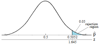
It looks like we should reject the null hypothesis because:
\[\hat{p}= 0.5172 > 0.5052\]
or equivalently since our test statistic Z = 5.49 is greater than 1.645.
Our Conclusion: We say there is sufficient evidence to conclude boys are more common than girls in the entire population.
\(p\)- value Approach
Next, let's state the procedure in terms of performing a proportion test using the p-value approach. The basic procedure is:
- State the null hypothesis H0 and the alternative hypothesis HA.
- Set the level of significance \(\alpha\).
- Calculate the test statistic:
\[z=\frac{\hat{p}-p_o}{\sqrt{\frac{p_0(1-p_0)}{n}}}\]
-
Calculate the p-value.
-
Make a decision. Check whether to reject the null hypothesis by comparing the p-value to \(\alpha\). If the p-value < \(\alpha\) then reject \(H_0\); otherwise do not reject \(H_0\).
Example S.6.2
Let's investigate by returning to our previous example. Again, we want to test
\(H_0: p=0.5\)
\(H_A: p>0.5\)
The test statistic
\[\begin{align} z &=\frac{\hat{p}-p_o}{\sqrt{\frac{p_0(1-p_0)}{n}}}\\
&=\frac{0.5172-0.5}{\sqrt{\frac{0.5(1-0.5)}{25468}}}\\
&= 5.49 \end{align}\]
The p-value is represented in the graph below:
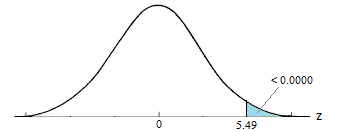
\[P = P(Z \ge 5.49) = 0.0000 \cdots \doteq 0\]
Our Conclusion: Because the p-value is smaller than the significance level \(\alpha = 0.05\), we can reject the null hypothesis. Again, we would say that there is sufficient evidence to conclude boys are more common than girls in the entire population at the \(\alpha = 0.05\) level.
As should always be the case, the two approaches, the critical value approach and the p-value approach lead to the same conclusion.
S.7 Self-Assess
S.7 Self-AssessWe suggest you...
- Review the concepts and methods on the pages in this section of this website.
- Download and Complete the Self-Assessment Exam.
- Determine your Score by reviewing the Self-Assessment Exam Solutions
A score below 70% suggests that the concepts and procedures that are covered in STAT 500 have not been mastered adequately. Students are strongly encouraged to take STAT 500, thoroughly review the materials that are covered in the sections above or take additional coursework that focuses on these foundations.
If you have struggled with the concepts and methods that are presented here, you will indeed struggle in any of the graduate-level courses included in the Master of Applied Statistics program above STAT 500 that expect and build on this foundation.
Note: These materials are NOT intended to be a complete treatment of the ideas and methods used in basic statistics. These materials and the accompanying self-assessment are simply intended as simply an 'early warning signal' for students. Also, please note that completing the self-assessment successfully does not automatically ensure success in any of the courses that use this foundation.
Calculus Review
Calculus ReviewSTAT 414 and STAT 415 are both required courses that were designed for the Master of Applied Statistics degree. These two courses provide the theoretical and mathematical foundations for the degree. Most students find these courses to be very challenging. The regularity of work and the rigorous nature of the concepts and methods can be daunting. For this reason, it is imperative that you have a working knowledge of multidimensional calculus as a prerequisite.
Many of our returning, working professional students report that they had taken the standard three-course calculus sequence (for example, MATH 140, MATH 141, and MATH 230) but these courses were completed a number of years ago. While it is relevant that you recognize these techniques it is expected that you can implement them.
An easy way to think about this may be in terms of an analogy. Perhaps as a child growing up you learned to play a musical instrument, and you might have been quite good. However, life has other plans for you and you realize that you have not picked up that instrument, or sat down at a piano for quite some time. While you might recognize the notes, the scales, or the keys to use, playing a song is not 'at your fingertips' as it once may have been. Students taking STAT 414 need to be ready to 'play the songs'! Re-learning the notes, the scales, and the keys at the same time as you are learning new concepts that involve these skills is often too much to handle and you get behind, and getting behind is no fun at all.
The review materials below are intended to provide a simple review of the calculus techniques most frequently used in the course. These are the topics that we want you to make sure that you have working knowledge of before you take STAT 414. They include:
- differentiation,
- integration,
- series,
- limits, and
- multivariate calculus.
We want our students to be successful! And we know that students that do not possess a working knowledge of these topics will struggle to participate successfully in STAT 414.
Review Materials
Are you ready? As a means of helping students assess whether or not what they currently know and can do will meet the expectations of instructors of STAT 414, the online program has put together a brief review of these concepts and methods. Each of these sections includes short self-assessment questions that will help you determine if this prerequisite knowledge is readily available for you to apply.
If you have struggled with the concepts and methods that are presented here, you will no doubt struggle in STAT 414 because this course expects and works off of this foundation.
Please Note: These materials are NOT intended to be a complete treatment of the ideas and methods used in multidimensional calculus. These materials and the self-assessment are simply intended as simply an 'early warning signal' for students. Also, please note that completing the self-assessment successfully does not automatically ensure success in any of the courses that use these foundation materials. Please keep in mind that this is a review only. It is not an exhaustive list of the material you need to have learned in your previous math classes. This review is meant only to be a simple guide of things you should remember.
C.1 Summations and Series
C.1 Summations and SeriesSummations and Series are an important part of discrete probability theory. We provide a brief review of some of the series used in STAT 414. While it is important to recall these special series, you should also take the time to practice. For a more in-depth review, there are links to Khan Academy.
Summations
First, it is important to review the notation. The symbol, \(\sum\), is a summation. Suppose we have the sequence, \(a_1, a_2, \cdots, a_n\), denoted \(\{a_n\}\), and we want to sum all their values. This can be written as
\[\sum_{i=1}^n a_i\]
Here are some special sums:
- \(\sum_{i=1}^n i=1+2+\cdots+n=\frac{n(n+1)}{2}\)
- \(\sum_{i=1}^n i^2=1^2+2^2+\cdots+n^2=\frac{n(n+1)(2n+1)}{6}\)
- The Binomial Theorem:
It is possible to expand any power of \(x+y\) to the sum
\[(x+y)^n=\sum_{i=0}^n {n \choose i} x^{n-i}y^i\]
where
\[{n\choose i}=\frac{n(n-1)(n-2)\cdots(n-i-1)}{i!}=\frac{n!}{(n-i)!i!}\]
Examples using the Binomial Theorem Video, (Khan Academy).
Series
When n is a finite number, the value of the sum can be easily determined. How do we find the sum when the sequence is infinite? For example, suppose we have an infinite sequence, \(a_1, a_2, \cdots\). The infinite series is denoted:
\[S=\sum_{i=1}^\infty a_i\]
For infinite series, we consider the partial sums. Some partial sums are
\[\begin{align*}
& S_1=\sum_{i=1}^1 a_i=a_1 \\
& S_2=\sum_{i=1}^2 a_i=a_1+a_2 \\
& S_3=\sum_{i=1}^3 a_i=a_1+a_2+a_3\\
& \vdots\\
& S_n=\sum_{i=1}^n a_i=a_1+a_2+\cdots+a_n
\end{align*}\]
An infinite series converges and has sum S if the sequence of partial sums, \(\{S_n\}\) converges to S. Thus, if
\[S=\lim_{n\rightarrow \infty} \{S_n\}\]
then the series converges to S. If \(\{S_n\}\) diverges, then the series diverges.
Review Convergence and Divergence of Series Video, (Khan Academy).
These are some of the special series used in STAT 414. It would be helpful to review more than what is listed below.
Geometric series
A geometric series has the form
\[S=\sum_{k=1}^\infty a r^{k-1}=a+ar+ar^2+ar^3+\cdots\]
where \(a\neq 0\). A geometric series converges to \(\frac{a}{1-r}\) if \(|r|<1\), but diverges if \(|r|\ge1\).
More examples and Explanation of the Geometric Series Video, (Khan Academy).
A special case of the geometric series
\[\frac{1}{1-x}=1+x+x^2+x^3+\cdots\]
for $-1<x<1$.
The Taylor (or Maclaurin) series of \(e^x\):
The series:
\[\sum_{i=0}^\infty \frac{x^i}{i!}=1+x+\frac{x^2}{2!}+\frac{x^3}{3!}+\cdots\]
for \(-1\le x\le 1\) converges to \(e^x\).
Review for the Taylor (or Maclaurin) Series Video, (Khan Academy).
Example C.1
\[S=\frac{1}{3}-\frac{1}{6}+\frac{1}{12}-\frac{1}{24}+\cdots=\sum_{x=0}^{\infty} \frac{1}{3(-2)^x}\]
This is a geometric series with \(a=\frac{1}{3}\) and \(r=-\frac{1}{2}\). Therefore, it converges to
\[\frac{a}{1-r}=\frac{\frac{1}{3}}{1+\frac{1}{2}}=\frac{2}{9}\]
C.2 Derivatives
C.2 DerivativesA complete review of derivatives would be lengthy. We try to touch on some topics that are used often in STAT 414 but not everything can be covered in the review. There are many good calculus books and websites to help you review. Students like the book Forgotten Calculus: A Refresher Course with Applications to Economics and Business by Barbara Lee Bleau, Ph.D. as a reference.
The definition of a derivative is
\[f^\prime(x)=\frac{d}{dx} f(x)=\lim_{h\rightarrow 0} \frac{f(x+h)-f(x)}{h}\]
The derivative is the slope of the tangent line to the graph of \(f(x)\), assuming the tangent line exists. You can find further explanations of derivatives on the web using websites like Khan Academy. Below are rules for determining derivatives and links for extra help.
- Common Derivatives and Rules
- Power Rule:
\(\frac{d}{dx}x^n=nx^{n-1}\) (Power Rule, Khan Academy) - \(\frac{d}{dx} \ln x=\frac{1}{x}\)
- \(\frac{d}{dx} a^x=a^x\ln a\)
- \(\frac{d}{dx} e^x=e^x\)
- Power Rule:
- Product rule
\(\begin{equation}\left[f(x)g(x)\right]^\prime=f^\prime(x)g(x)+f(x)g^\prime(x)\end{equation}\) (Product Rule, Khan Academy) - Quotient rule
\(\begin{equation} \left[\frac{f(x)}{g(x)}\right]^\prime=\frac{g(x)f^\prime(x)-f(x)g^\prime(x)}{\left(g(x)\right)^2}\end{equation}\) (Quotient Rule, Khan Academy) - Chain Rule
Let \(y=f(g(x))\) where f and g are functions, g is differentiable at x, and f is differentiable at \(g(x)\). Then the derivative of y is \(f^\prime(g(x))g^\prime(x)\). (Chain Rule, Khan Academy) - L'Hopital's Rule
- For the type \(0/0\): Suppose that \(\lim_{x\rightarrow u} f(x)=0\) and \(\lim_{x\rightarrow u} g(x)=0\). If \(\lim_{x\rightarrow u}\left[\frac{f^\prime(x)}{g^\prime(x)}\right]\) exists in either the finite or infinite sense, then\[\begin{equation}\lim_{x\rightarrow u} \frac{f(x)}{g(x)}=\lim_{x\rightarrow u} \frac{f^\prime(x)}{g^\prime(x)}=\frac{\lim_{x\rightarrow u} f^\prime(x)}{\lim_{x\rightarrow u} g^\prime(x)}\end{equation}\]
- For the type \(\infty/\infty\): Suppose that \(\lim_{x\rightarrow u} |f(x)|=\infty\) and \(\lim_{x\rightarrow u} |g(x)|=\infty\). If \(\lim_{x\rightarrow u}\left[\frac{f^\prime(x)}{g^\prime(x)}\right]\) exists in either the finite or infinite sense, then\[\begin{equation}\lim_{x\rightarrow u} \frac{f(x)}{g(x)}=\lim_{x\rightarrow u} \frac{f^\prime(x)}{g^\prime(x)}=\frac{\lim_{x\rightarrow u} f^\prime(x)}{\lim_{x\rightarrow u} g^\prime(x)}\end{equation}\]
- Other indeterminate forms can also be solved using L'Hopital's Rule, such as \(0^0\) and \(\infty^0\). It would be a good idea for review the uses of L'Hopital's Rule. (L'Hopital's Rule, Khan Academy)
Example C.2.1
Find the derivative of \(f(x)\) for the following:
- \(f(x)=10x^9-5x^5+7x^3-9\)
- \(f(x)=\dfrac{x}{x^2+5}\)
- \(f(x)=\dfrac{1}{\sqrt{x}}\)
- \(f^\prime(x)=90x^8-25x^4+21x^2\)
- Using the Quotient Rule, \(f^\prime(x)=\dfrac{x^2+5-x(2x)}{(x^2+5)^2}=\dfrac{-x^2+5}{(x^2+5)^2}\)
- Using the Power Rule, \(f^\prime(x)=-\dfrac{1}{2x\sqrt{x}}\)
Example C.2.2
C.3 Integrals
C.3 IntegralsAs with the review of Derivatives, it would be challenging to include a full review of Integrals. In this review, we try to include the most common integrals and rules used in STAT 414. There are many helpful websites and texts out there to help you review. We have provided links to Khan Academy for you to take a look at if you have difficulty recalling these methods.
For a function, \(f(x)\), its indefinite integral is:
\[\int f(x)\; dx=F(x)+C, \qquad \text{where } F^\prime(x)=f(x)\]
We provide a short list of common integrals and rules that are used in STAT 414. It is important to have a lot of practice and keep these skills fresh.
Common Integrals and Rules
- \(\int_a^a f(x)dx=0\)
- \(\int_a^b f(x)d(x)=-\int_b^a f(x)d(x)\)
- \(\int x^rdx=\frac{x^{r+1}}{r+1}+C\)
The Fundamental Theorem of Calculus:
Let \(f\) be integrable on \([a,b]\) and let \(F\) be any antiderivative of \(f\) there. Then, \(\int_a^b f(x)d(x)=F(b)-F(a)\). (FTC, Khan Academy)
- \(\int x^n dx=\dfrac{1}{n+1}x^{n+1}+C, \;\;n\neq(-1)\)
- \(\int \dfrac{1}{x}dx=\ln |x| +C\)
- \(\int e^x dx=e^x +C\)
Integration Using Substitution:
Let \(g\) have a continuous derivative on \([a,b]\) and let \(f\) be continuous on the range of \(g\). Then
\[\begin{equation}
\int_a^b f\left(g(x)\right)g^\prime(x)dx=\int_{g(a)}^{g(b)}f(u)du
\end{equation}\]
where \(u=g(x)\). (u-Substitution, Khan Academy)
Integration by Parts
\[\begin{equation}
\int_a^b udv=\left[uv\right]_a^b-\int_a^b vdu \end{equation}\].
(Integration by Parts, Khan Academy)
Example C.3.1
Integrate the following function from 0 to $t$
\[f(x)=\dfrac{2}{1000^2}xe^{-(x/1000)^2}\]
\[\int_0^t \frac{2}{1000^2}xe^{-(x/1000)^2} dx\label{eqn1}\]
Let \(u=\left(\frac{x}{1000}\right)^2\). Then \(du=\frac{2}{1000^2}xdx\). The equation becomes...
\[\begin{align*}
&= \int_0^{\left(\frac{t}{1000}\right)^2} e^{-u}du =-e^{-u}|_{0}^{\left(\frac{t}{1000}\right)^2}\\
&= -e^{-\left(\frac{t}{1000}\right)^2}-(-1)=1-e^{-\left(\frac{t}{1000}\right)^2}.
\end{align*}\]
Example C.3.2
Integrate the following:
\[\int_0^5 x^2e^{-x}dx\]
Let us begin by setting up integration by parts. Let
\[\begin{align*}
& u=x^2 \qquad dv=e^{-x}dx\\
& du=2xdx \qquad v=-e^{-x}
\end{align*}\]
Then
\[\begin{align*}
uv|_0^5-\int_0^5 vdu &=-x^2e^{-x}|_0^5+2\int_0^5xe^{-x}dx\\
&= -x^2e^{-x}|_0^5+2\left[-xe^{-x}|_0^5+\int_0^5 e^{-x}dx\right]\\
&= -x^2e^{-x}|_0^5+2\left[-xe^{-x}|_0^5-e^{-x}|_0^5\right]\approx 1.75
\end{align*}\]
Example C.3.3
Integrate the following from \(-\infty\) to \(\infty\).
\[f(y)=\frac{1}{2}e^{-|y|+ty}, \;\; \text{ for } -\infty<y<\infty\]
\begin{align*}
\int_{-\infty}^{\infty} \frac{1}{2} e^{ty-|y|}dy &= \int_{-\infty}^0 \frac{1}{2}e^{y+ty}dy+\int_0^{\infty} \frac{1}{2}e^{-y+ty}dy\\
& = \int_{-\infty}^0 \frac{1}{2}e^{y(1+t)}dy+\int_0^{\infty} \frac{1}{2}e^{-y(1-t)}dy\\
& = \frac{1}{2(1+t)}+ \frac{1}{2(1-t)}=\frac{1}{2}\left(\frac{1-t+t+1}{(1+t)(1-t)}\right)\\
& =\frac{1}{(1-t)(1+t)}
\end{align*}
C.4 Multivariable Calculus
C.4 Multivariable CalculusIn this review, we present a couple of the more important Multivariable Calculus methods commonly used in STAT 414, mainly for Exam 4 and the Final Exam. While this is not a complete review, you should use this to refresh your memory and guide you to where you need to spend time reviewing. As always, practice is key!
First, multivariable calculus involves functions of several variables. For simplicity, we focus on the functions of two variables. You can find information on the web or in other texts to review in more detail if you need.
Partial Derivatives
Let's begin with Partial Derivatives. Suppose we have the function \(f(x,y)\). The partial derivative with respect to x would be
\[f_x(x,y)=\lim_{h\rightarrow 0} \frac{f(x-h, y)}{x-h}\]
Similarly, the partial derivative of \(f(x,y)\) with respect to \(y\) would be
\[f_y(x,y)=\lim_{h\rightarrow 0} \frac{f(x, y-h)}{y-h}\]
The notation for partial derivatives is not the same for all texts. You should be able to recognize the different forms. The notation, for example, for the partial derivative of $f(x,y)$, with respect to $x$, could be denoted as:
\[f_x(x,y)=\frac{\partial}{\partial x}f(x, y)=\frac{\partial f}{\partial x}\]
Derivatives of Multivariable Functions Video, (Khan Academy)
Double Integrals
Integrating over regions will be important in STAT 414. Suppose we have the function \(f(x,y)\), the over the region R, would be:
\[\int \int_R f(x,y)\; dx dy\]
Consider the rectangular region defined by \(a\le x\le b\) and \(c\le y\le d\), or \(R=[a,b]\times[c, d]\). Then the iterated integral would be:
\( \int_c^d \left[\int_a^b f(x,y) dx\right] dy=\int_a^b \left[\int_c^d f(x,y) dy\right] dx \)
When the region is not rectangular, things can get complicated. It is important to draw out the support space and consider the region when building these double integrals.
Double Integrals Video, (Khan Academy)
Example C.4.1
First, let's find the partial of x. To do this, we consider y as a constant.
\[\dfrac{\partial f}{\partial x}=-\dfrac{2}{x^3}-y\]
Now, let's find \(\dfrac{\partial f}{\partial y}\).
\[\dfrac{\partial f}{\partial y}=\dfrac{3}{\sqrt{y}}-x\]
Example C.4.2
Integrate \(f(x,y) =24xy\). For \(0< x < 1, 0 <y<1\) and \(x+y < 1\) over the space where \(x+y<\dfrac{1}{2}\).
\begin{align*}
\int_0^{1/2}\int_{0}^{1/2-y} 24xy\; dx \; dy &=\int_0^{1/2} 12y^3-12y^2+3y\; dy\\
& = 3y^4-4y^3+\dfrac{3}{2}y^2|_0^{1/2}\\&=3\left(\dfrac{1}{2}\right)^4-4\left(\dfrac{1}{2}\right)^3+\dfrac{3}{2}\left(\dfrac{1}{2}\right)^2\\
& = \dfrac{1}{16}
\end{align*}
Matrix Algebra Review
Matrix Algebra ReviewMatrix Algebra: A Review
The Prerequisites Checklist page on the Department of Statistics website lists a number of courses that require a working knowledge of Matrix algebra as a prerequisite. Students who do not have this foundation or have not reviewed this material within the past couple of years will struggle with the concepts and methods that build on this foundation. The courses that require this foundation include:
- STAT 414 - Introduction to Probability Theory
- STAT 501 - Regression Methods
- STAT 504 - Analysis of Discrete Data
- STAT 505 - Applied Multivariate Statistical Analysis
Review Materials
Many of our returning, working professional students report that they had taken courses that included matrix algebra topics but often these courses were taken a number of years ago. As a means of helping students assess whether or not what they currently know and can do will meet the expectations of instructors in the courses above, the online program has put together a brief review of these concepts and methods. This is then followed by a short self-assessment exam that will help give you an idea if you still have the necessary background.
Self-Assessment Procedure
- Review the concepts and methods on the pages in this section of this website. Note the courses that certain sections are aligned with as prerequisites:
STAT 414 STAT 501 STAT 504 STAT 505 M.1 - Matrix Definitions Required Required Required Required M.2 - Matrix Arithmetic Required Required Required Required M.3 - Matrix Properties Required Required Required Required M.4 - Matrix Inverse Required Required Required Required M.5 - Advanced Topics Recommended Recommended Recommended 5.1, 5.4, Required
5.2, 5.3, Recommended - Download and complete the Self-Assessment Exam
- Review the Self-Assessment Exam Solutions and determine your score.
Students who score below 70% (fewer than 21 questions correct) should consider further review of these materials and are strongly encouraged to take a course like MATH 220 or an equivalent course at a local college or community college.
If you have struggled with the concepts and methods that are presented here, you will indeed struggle in the courses above that expect this foundation.
Please Note: These materials are NOT intended to be a complete treatment of the ideas and methods used in Matrix algebra. These materials and the self-assessment are simply intended as simply an 'early warning signal' for students. Also, please note that completing the self-assessment successfully does not automatically ensure success in any of the courses that use these foundation materials.
M.1 Matrix Definitions
M.1 Matrix Definitions- Matrix
-
A matrix is a rectangular collection of numbers. Generally, matrices are denoted as bold capital letters. For example:
\[A = \begin{pmatrix} 1 & -5 & 4\\
2 & 5 & 3 \end{pmatrix}\]
A is a matrix with two rows and three columns. For that reason, it is called a 2 by 3 matrix. This is called the dimension of a matrix.
- Dimension
-
The dimension of a matrix is expressed as number of rows × number of columns. So,
\[B = \begin{pmatrix} 1 & -5 & 4 \\ 5 & 3 & -8 \\ 1 & 5 & 4 \\ 2 & 5 & 3 \end{pmatrix}\]
B is a 4 × 3 matrix. It is common to refer to elements in a matrix by subscripts, like so.
\[B = \begin{pmatrix} b_{1,1} & b_{1,2} & b_{1,3}\\ b_{2,1} & b_{2,2} & b_{2,3}\\ b_{3,1} & b_{3,2} & b_{3,3}\\ b_{4,1} & b_{4,2} & b_{4,3} \end{pmatrix}\]
With the row first and the column second. So in this case, \(b_{2,1} = 5\) and \(b_{1,3} =4\).
- Vector
-
A vector is a matrix with only one row (called a row vector) or only one column (called a column vector). For example:
\[C = \begin{pmatrix} 2 & 7 & -3 & 5 \end{pmatrix}\]
C is a 4 dimensional row vector.
\[D = \begin{pmatrix} 2 \\9 \\-3 \\3\\ 6\\ \end{pmatrix}\]
D is a 5 dimensional column vector. An "ordinary" number can be thought of as a 1 × 1 matrix, also known as a scalar. Some examples of scalars are shown below:
\[ E = \pi \]
\[ F = 6 \]
M.2 Matrix Arithmetic
M.2 Matrix ArithmeticTranspose a Matrix
To take the transpose of a matrix, simply switch the rows and column of a matrix. The transpose of \(A\) can be denoted as \(A'\) or \(A^T\).
For example
\[A = \begin{pmatrix} 1 & -5 & 4 \\ 2 & 5 & 3 \end{pmatrix}\]
\[A' = A^T = \begin{pmatrix} 1 & 2\\ -5 & 5\\ 4 & 3 \end{pmatrix}\]
If a matrix is its own transpose, then that matrix is said to be symmetric. Symmetric matrices must be square matrices, with the same number of rows and columns.
One example of a symmetric matrix is shown below:
\[ A = \begin{pmatrix} 1 & -5 & 4 \\ -5 & 7 & 3\\ 4 & 3 & 3 \end{pmatrix} = A' = A^T \]
Matrix Addition
To perform matrix addition, two matrices must have the same dimensions. This means they must have the same number of rows and columns. In that case simply add each individual components, like below.
For example
\[A + B = \begin{pmatrix} 1 & -5 & 4 \\ 2 & 5 & 3 \end{pmatrix} + \begin{pmatrix} 8 & -3 & -4 \\ 4 & -2 & 9 \end{pmatrix} = \begin{pmatrix} 1 + 8 & -5 - 3 & 4 - 4 \\ 2 + 4 & 5 -2 & 3 + 9 \end{pmatrix} = \begin{pmatrix} 9 & -8 & 0\\ 6 & 3 & 12 \end{pmatrix}\]
Matrix addition does have many of the same properties as "normal" addition.
\[A + B = B + A\]
\[A + (B + C) = (A + B) + C\]
In addition, if one wishes to take the transpose of the sum of two matrices, then
\[A^T + B^T = (A+B)^T \]
Matrix Scalar Multiplication
To multiply a matrix by a scalar, also known as scalar multiplication, multiply every element in the matrix by the scalar.
For example...
\[ 6*A = 6 * \begin{pmatrix} 1 & -5 & 4\\ 2 & 5 & 3 \end{pmatrix} = \begin{pmatrix} 6 * 1 & 6 *-5 & 6 * 4\\ 6 * 2 & 6 *5 & 6 * 3 \end{pmatrix} = \begin{pmatrix} 6 & -30 & 24 \\ 12 & 30 & 18 \end{pmatrix}\]
To multiply two vectors with the same length together is to take the dot product, also called inner product. This is done by multiplying every entry in the two vectors together and then adding all the products up.
For example, for vectors x and y, the dot product is calculated below
\[ x \cdot y = \begin{pmatrix} 1 & -5 & 4 \end{pmatrix} * \begin{pmatrix} 4 & -2 & 5 \end{pmatrix} = 1*4 + (-5)*(-2) + 4*5 = 4+10+20 = 34\]
Matrix Multiplication
To perform matrix multiplication, the first matrix must have the same number of columns as the second matrix has rows. The number of rows of the resulting matrix equals the number of rows of the first matrix, and the number of columns of the resulting matrix equals the number of columns of the second matrix. So a 3 × 5 matrix could be multiplied by a 5 × 7 matrix, forming a 3 × 7 matrix, but one cannot multiply a 2 × 8 matrix with a 4 × 2 matrix. To find the entries in the resulting matrix, simply take the dot product of the corresponding row of the first matrix and the corresponding column of the second matrix.
For example
\[ C*D = \begin{pmatrix} 3 & -9 & -8\\ 2 & 4 & 3 \end{pmatrix} * \begin{pmatrix} 7 & -3\\ -2 & 3\\ 6 & 2 \end{pmatrix} \]
\[ C*D = \begin{pmatrix} 3*7 + (-9)*(-2) + (-8)*6 & 3*(-3) + (-9)*3 + (-8)*2 \\ 2*7 + 4*(-2) + 3*6 & 2*(-3) + 4*3 + 3*2 \end{pmatrix}\]
\[ C*D = \begin{pmatrix} 21 + 18 - 48 & - 9 - 27 - 16 \\14 - 8 + 18 & - 6 + 12 + 6 \end{pmatrix} = \begin{pmatrix} -9 & - 52\\ 24 & 12 \end{pmatrix} \]
Matrix multiplication has some of the same properties as "normal" multiplication , such as
\[ A(BC) = (AB)C\]
\[A(B + C) = AB + AC\]
\[(A + B)C = AC + BC\]
However matrix multiplication is not commutative. That is to say A*B does not necessarily equal B*A. In fact, B*A often has no meaning since the dimensions rarely match up. However, you can take the transpose of matrix multiplication. In that case \((AB)^T = B^T A^T\).
M.3 Matrix Properties
M.3 Matrix PropertiesIdentity Matrices
An identity matrix is a square matrix where every diagonal entry is 1 and all the other entries are 0. The following two matrices are identity matrices and diagonal matrices.
\[ I_3 = \begin{pmatrix} 1 & 0 & 0 \\0 & 1 & 0\\ 0 & 0 & 1 \end{pmatrix} \]
\[ I_4 = \begin{pmatrix} 1 & 0 & 0 & 0\\ 0 & 1 & 0 & 0\\ 0 & 0 & 1 & 0\\ 0 & 0 & 0 & 1 \end{pmatrix} \]
They are called identity matrices because any matrix multiplied with an identity matrix equals itself. The diagonal entries of a matrix are the entries where the column and row number are the same. \(a_{2,2}\) is a diagonal entry but \(a_{3,5}\) is not. The trace of an n × n matrix is the sum of all the diagonal entries. In other words, for n × n matrix A, \(trace(A) = tr(A) = \sum_{i=1}^{n} a_{i,i}\) For example:
\[ trace(F) = tr(F) = tr \begin{pmatrix} 1 & 3 & 3\\ 0 & 6 & 7\\ -5 & 0 & 1 \end{pmatrix} = 1 + 6 + 1 = 8 \]
The trace has some useful properties, namely that for same size square matrices A and B and scalar c,
\[ tr(A) = tr(A^T)\] \[ tr(A + B) = tr(B + A) = tr(A) + tr(B)\] \[ tr(AB) = tr(BA)\] \[ tr(cA) = c*tr(A)\]
Determintants
The determinate of a square, 2 × 2 matrix A is
\[ det(A) = |A| = \begin{vmatrix} a_{1,1} & a_{1,2} \\ a_{2,1} & a_{2,2} \end{vmatrix} = a_{1,1} * a_{2,2} - a_{1,2}*a_{2,1}\]
For example
\[ det(A) = |A| = \begin{vmatrix} 5 & 2 \\ 7 & 2 \end{vmatrix} = 5*2 - 2*7 = -4\]
For a 3 × 3 matrix B, the determinate is
\[det(B) = |B| = \begin{vmatrix} b_{1,1} & b_{1,2} & b_{1,3}\\ b_{2,1} & b_{2,2} & b_{2,3}\\ b_{3,1} & b_{3,2} & b_{3,3} \end{vmatrix} = b_{1,3} \begin{vmatrix} b_{2,1} & b_{2,2}\\ b_{3,1} & b_{3,2} \end{vmatrix} - b_{2,3} \begin{vmatrix} b_{1,1} & b_{1,2}\\ b_{3,1} & b_{3,2} \end{vmatrix} + b_{3,3} \begin{vmatrix} b_{1,1} & b_{1,2} \\b_{2,1} & b_{2,2} \end{vmatrix}\]
\[ det(B) = b_{1,3}(b_{2,1} b_{3,2} - b_{2,2} b_{3,1} ) - b_{2,3}(b_{1,1} b_{3,2} - b_{1,2} b_{3,1} ) + b_{3,3}(b_{1,1} b_{2,2} - b_{1,2} b_{2,1} ) \]
For example:
\[det(B) = |B| = \begin{vmatrix} 4 & 0 & -1\\2 & -2 & 3 \\ 7 & 5 & 0 \end{vmatrix} = -1 \begin{vmatrix} 2 & -2\\ 7 & 5 \end{vmatrix} - 3 \begin{vmatrix} 4 & 0 \\7 & 5 \end{vmatrix} + 0 \begin{vmatrix} 4 & 0 \\ 2 & -2 \end{vmatrix}\]
\[ det(B) = -1 (2*5 - (-2)*7) + 3(4*5 - 0 *7) - 0 (4*(-2) - 0 * 2) = -1*24 - 3*20 + 0 *(-8) = -24 - 60 = -84 \]
In general, to find the determinate of a n \(\times\) n matrix, choose a row or column like column 1, and take the determinates of the "minor" matrices inside the original matrix, like so:
\[det(C) = |C| = \begin{vmatrix} c_{1,1} & c_{1,2} & \ldots & c_{1,n}\\ c_{2,1} & c_{2,2} & \ldots & c_{2,n}\\ \vdots & \vdots & \ddots & \vdots \\c_{n,1} & c_{.,2} & \ldots & c_{n,n} \end{vmatrix}\]
\[det(C) = (-1)^{1+1} c_{1,1} \begin{vmatrix} c_{2,2} & \ldots & c_{2,n}\\ \vdots & \ddots & \vdots \\ c_{n,2} & \ldots & c_{n,n} \end{vmatrix} + (-1)^{2+1} c_{2,1} \begin{vmatrix} c_{1,2} & \ldots & c_{1,n}\\ c_{3,2} & \ldots & c_{3,n}\\ \vdots & \ddots & \vdots\\ c_{n,2} & \ldots & c_{n,n} \end{vmatrix} + \ldots\]
\[ \ldots + (-1)^{n+1} c_{n,1} \begin{vmatrix} c_{1,2} & \ldots & c_{1,n}\\ \vdots & \ddots & \vdots \\ c_{n-1,2} & \ldots & c_{n-1,n} \end{vmatrix} \]
This is known as Laplace's formula,
\[ det(A) = \sum_{j=1}^{n} (-1)^{i+j} a_{i,j} det(A_{-i,-j}) = \sum_{i=1}^{n} (-1)^{i+j} a_{i,j} det(A_{-i,-j}) \]
For any i, j, where \(A_{-i,-j}\) is matrix A with row i and column j removed. This formula works whether one goes by rows, using the first formulation, or by columns, using the second formulation. It is easiest to use Laplace's formula when one chooses the row or column with the most zeroes.
Matrix Determinant Properties
The matrix determinate has some interesting properties.
\[det(I) = 1\]
where I is the identity matrix.
\[det(A) = det(A^T)\]
If A and B are square matrices with the same dimensions, then
\[ det(AB) = det(A)*det(B)\] and if A is a n × n square matrix and c is a scalar, then
\[ det(cA) = c^n det(A)\]
M.4 Matrix Inverse
M.4 Matrix Inverse- Inverse of a Matrix
-
The matrix B is the inverse of matrix A if \(AB = BA = I\). This is often denoted as \(B = A^{-1}\) or \(A = B^{-1}\). When taking the inverse of the product of two matrices A and B,
\[(AB)^{-1} = B^{-1} A^{-1}\]
When taking the determinate of the inverse of the matrix A,
\[ det(A^{-1}) = \frac{1}{det(A)} = det(A)^{-1}\]
Note that not all matrices have inverses. For a matrix A to have an inverse, that is to say for A to be invertible, A must be a square matrix and \(det(A) \neq 0\). For that reason, invertible matrices are also called nonsingular matrices.
Two examples are shown below
\[ det(A) = \begin{vmatrix} 4 & 5 \\ -2 & 1 \end{vmatrix} = 4*1-5*-2 = 14 \neq 0 \]
\[ det(C) = \begin{vmatrix} 1 & 2 & -1\\ 5 & 3 & 2 \\ 6 & 0 & 6 \end{vmatrix} = -2 \begin{vmatrix} 5 & 2 \\ 6 & 6 \end{vmatrix} + 3 \begin{vmatrix} 1 & -1\\ 6 & 6 \end{vmatrix} + 0 \begin{vmatrix} 1 & -1\\ 5 & 2 \end{vmatrix}\]
\[ det(C)= - 2(5*6-2*6) + 3(1*6-(-1)*6) - 0(1*2-(-1)*5) = 0 \]
So C is not invertible, because its determinate is zero. However, A is an invertible matrix, because its determinate is nonzero. To calculate that matrix inverse of a 2 × 2 matrix, use the below formula.
\[ A^{-1} = \begin{pmatrix} a_{1,1} & a_{1,2}\\ a_{2,1} & a_{2,2} \end{pmatrix} ^{-1} = \frac{1}{det(A)} \begin{pmatrix} a_{2,2} & -a_{1,2} \\ -a_{2,1} & a_{1,1} \end{pmatrix} = \frac{1}{a_{1,1} * a_{2,2} - a_{1,2}*a_{2,1}} \begin{pmatrix} a_{2,2} & -a_{1,2} \\ -a_{2,1} & a_{1,1} \end{pmatrix}\]
For example
\[ A^{-1} = \begin{pmatrix} 4 & 5 \\ -2 & 1 \end{pmatrix} ^{-1} = \frac{1}{det(A)} \begin{pmatrix} 1 & -5 \\ 2 & 4 \end{pmatrix} = \frac{1}{4*1 - 5*(-2)} \begin{pmatrix} 1 & -5 \\ 2 & 4 \end{pmatrix} = \begin{pmatrix} \frac{1}{14} & \frac{-5}{14} \\ \frac{2}{14} & \frac{4}{14} \end{pmatrix}\]
For finding the matrix inverse in general, you can use Gauss-Jordan Algorithm. However, this is a rather complicated algorithm, so usually one relies upon the computer or calculator to find the matrix inverse.
M.5 Advanced Matrix Properties
M.5 Advanced Matrix Properties- Orthogonal Vectors
-
Two vectors, x and y, are orthogonal if their dot product is zero.
For example
\[ e \cdot f = \begin{pmatrix} 2 & 5 & 4 \end{pmatrix} * \begin{pmatrix} 4 \\ -2 \\ 5 \end{pmatrix} = 2*4 + (5)*(-2) + 4*5 = 8-10+20 = 18\]
Vectors e and f are not orthogonal.
\[ g \cdot h = \begin{pmatrix} 2 & 3 & -2 \end{pmatrix} * \begin{pmatrix} 4 \\ -2 \\ 1 \end{pmatrix} = 2*4 + (3)*(-2) + (-2)*1 = 8-6-2 = 0\]
However, vectors g and h are orthogonal. Orthogonal can be thought of as an expansion of perpendicular for higher dimensions. Let \(x_1, x_2, \ldots , x_n\) be m-dimensional vectors. Then a linear combination of \(x_1, x_2, \ldots , x_n\) is any m-dimensional vector that can be expressed as
\[ c_1 x_1 + c_2 x_2 + \ldots + c_n x_n \]
where \(c_1, \ldots, c_n\) are all scalars. For example:
\[x_1 =\begin{pmatrix}
3 \\
8 \\
-2
\end{pmatrix},
x_2 =\begin{pmatrix}
4 \\
-2 \\
3
\end{pmatrix}\]
\[y =\begin{pmatrix}
-5 \\
12 \\
-8
\end{pmatrix} = 1*\begin{pmatrix}
3 \\
8 \\
-2
\end{pmatrix} + (-2)* \begin{pmatrix}
4 \\
-2 \\
3
\end{pmatrix} = 1*x_1 + (-2)*x_2\]
So y is a linear combination of \(x_1\) and \(x_2\). The set of all linear combinations of \(x_1, x_2, \ldots , x_n\) is called the span of \(x_1, x_2, \ldots , x_n\). In other words
\[ span(\{x_1, x_2, \ldots , x_n \} ) = \{ v| v= \sum_{i = 1}^{n} c_i x_i , c_i \in \mathbb{R} \} \]
A set of vectors \(x_1, x_2, \ldots , x_n\) is linearly independent if none of the vectors in the set can be expressed as a linear combination of the other vectors. Another way to think of this is a set of vectors \(x_1, x_2, \ldots , x_n\) are linearly independent if the only solution to the below equation is to have \(c_1 = c_2 = \ldots = c_n = 0\), where \(c_1 , c_2 , \ldots , c_n \) are scalars, and \(0\) is the zero vector (the vector where every entry is 0).
\[ c_1 x_1 + c_2 x_2 + \ldots + c_n x_n = 0 \]
If a set of vectors is not linearly independent, then they are called linearly dependent.
Example M.5.1
\[ x_1 =\begin{pmatrix} 3 \\ 4 \\ -2 \end{pmatrix}, x_2 =\begin{pmatrix} 4 \\ -2 \\ 2 \end{pmatrix}, x_3 =\begin{pmatrix} 6 \\ 8 \\ -2 \end{pmatrix} \]
Does there exist a vector c, such that,
\[ c_1 x_1 + c_2 x_2 + c_3 x_3 = 0 \]
To answer the question above, let:
\begin{align} 3c_1 + 4c_2 +6c_3 &= 0,\\ 4c_1 -2c_2 + 8c_3 &= 0,\\ -2c_1 + 2c_2 -2c_3 &= 0 \end{align}
Solving the above system of equations shows that the only possible solution is \(c_1 = c_2 = c_3 = 0\). Thus \(\{ x_1 , x_2 , x_3 \}\) is linearly independent. One way to solve the system of equations is shown below. First, subtract (4/3) times the 1st equation from the 2nd equation.
\[-\frac{4}{3}(3c_1 + 4c_2 +6c_3) + (4c_1 -2c_2 + 8c_3) = -\frac{22}{3}c_2 = -\frac{4}{3}0 + 0 = 0 \Rightarrow c_2 = 0 \]
Then add the 1st and 3 times the 3rd equations together, and substitute in \(c_2 = 0\).
\[ (3c_1 + 4c_2 +6c_3) + 3*(-2c_1 + 2c_2 -2c_3) = -3c_1 + 10 c_2 = -3c_1 + 10*0 = 0 + 3*0 = 0 \Rightarrow c_1 = 0 \]
Now, substituting both \(c_1 = 0\) and \(c_2 = 0\) into equation 2 gives.
\[ 4c_1 -2c_2 + 8c_3 = 4*0 -2*0 + 8c_3 = 0 \Rightarrow c_3 = 0 \]
So \(c_1 = c_2 = c_3 = 0\), and \(\{ x_1 , x_2 , x_3 \}\) are linearly independent.
Example M.5.2
\[ x_1 =\begin{pmatrix} 1 \\ -8 \\ 8 \end{pmatrix}, x_2 =\begin{pmatrix} 4 \\ -2 \\ 2 \end{pmatrix}, x_3 =\begin{pmatrix} 1 \\ 3 \\ -2 \end{pmatrix} \]
In this case \(\{ x_1 , x_2 , x_3 \}\)are linearly dependent, because if \(c = (-1, 1, -2)\), then
\[c^T X = \begin{pmatrix}
-1 \\
1\\
-2
\end{pmatrix} \begin{pmatrix}
x_1 & x_2 & x_3
\end{pmatrix} = -1 \begin{pmatrix}
1 \\
-8\\
8
\end{pmatrix}+ 1
\begin{pmatrix}
4 \\
-2\\
2
\end{pmatrix} - 2 \begin{pmatrix}
1 \\
3 \\
-2
\end{pmatrix} =
\begin{pmatrix}
-1*1 +1*4-2*1 \\
-1*-8+1*-2-2*3 \\
-1*8+1*2-2*-2
\end{pmatrix}=
\begin{pmatrix}
0 \\
0 \\
0
\end{pmatrix}
\]
- Norm of a vector or matrix
-
The norm of a vector or matrix is a measure of the "length" of said vector or matrix. For a vector x, the most common norm is the \(\mathbf{L_2}\) norm, or Euclidean norm. It is defined as
\[ \| x \| = \| x \|_2 = \sqrt{ \sum_{i=1}^{n} x_i^2 } \]
Other common vector norms include the \(\mathbf{L_1}\) norm, also called the Manhattan norm and Taxicab norm.
\[ \| x \|_1 = \sum_{i=1}^{n} |x_i| \]
Other common vector norms include the Maximum norm, also called the Infinity norm.
\[ \| x \|_\infty = max( |x_1| ,|x_2|, \ldots ,|x_n|) \]
The most commonly used matrix norm is the Frobenius norm. For a m × n matrix A, the Frobenius norm is defined as:
\[ \| A \| = \| A \|_F = \sqrt{ \sum_{i=1}^{m} \sum_{j=1}^{n} x_{i,j}^2 } \]
- Quadratic Form of a Vector
-
The quadratic form of the vector x associated with matrix A is
\[ x^T A x = \sum_{i = 1}^{m} \sum_{j=1}^{n} a_{i,j} x_i x_j \]
A matrix A is Positive Definite if for any non-zero vector x, the quadratic form of x and A is strictly positive. In other words, \(x^T A x > 0\) for all nonzero x.
A matrix A is Positive Semi-Definite or Non-negative Definite if for any non-zero vector x, the quadratic form of x and A is non-negative . In other words, \(x^T A x \geq 0\) for all non-zero x. Similarly,
A matrix A is Negative Definite if for any non-zero vector x, \(x^T A x < 0\). A matrix A is Negative Semi-Definite or Non-positive Definite if for any non-zero vector x, \(x^T A x \leq 0\).
M.6 Range, Nullspace and Projections
M.6 Range, Nullspace and Projections- Range of a matrix
-
The range of m × n matrix A, is the span of the n columns of A. In other words, for
\[ A = [ a_1 a_2 a_3 \ldots a_n ] \]
where \(a_1 , a_2 , a_3 , \ldots ,a_n\) are m-dimensional vectors,
\[ range(A) = R(A) = span(\{a_1, a_2, \ldots , a_n \} ) = \{ v| v= \sum_{i = 1}^{n} c_i a_i , c_i \in \mathbb{R} \} \]
The dimension (number of linear independent columns) of the range of A is called the rank of A. So if 6 × 3 dimensional matrix B has a 2 dimensional range, then \(rank(A) = 2\).
For example
\[C =\begin{pmatrix}
1 & 4 & 1\\
-8 & -2 & 3\\
8 & 2 & -2
\end{pmatrix} = \begin{pmatrix}
x_1 & x_2 & x_3
\end{pmatrix}= \begin{pmatrix}
y_1 \\
y_2\\
y_3
\end{pmatrix}\]
C has a rank of 3, because \(x_1\), \(x_2\) and \(x_3\) are linearly independent.
- Nullspace
- p>The nullspace of a m \(\times\) n matrix is the set of all n-dimensional vectors that equal the n-dimensional zero vector (the vector where every entry is 0) when multiplied by A. This is often denoted as
\[N(A) = \{ v | Av = 0 \}\]
The dimension of the nullspace of A is called the nullity of A. So if 6 \(\times\) 3 dimensional matrix B has a 1 dimensional range, then \(nullity(A) = 1\).
The range and nullspace of a matrix are closely related. In particular, for m \(\times\) n matrix A,
\[\{w | w = u + v, u \in R(A^T), v \in N(A) \} = \mathbb{R}^{n}\]
\[R(A^T) \cap N(A) = \phi\]
This leads to the rank--nullity theorem, which says that the rank and the nullity of a matrix sum together to the number of columns of the matrix. To put it into symbols:
\[A \in \mathbb{R}^{m \times n} \Rightarrow rank(A) + nullity(A) = n\]
For example, if B is a 4 \(\times\) 3 matrix and \(rank(B) = 2\), then from the rank--nullity theorem, on can deduce that
\[rank(B) + nullity(B) = 2 + nullity(B) = 3 \Rightarrow nullity(B) = 1\]
- Projection
The projection of a vector x onto the vector space J, denoted by Proj(X, J), is the vector \(v \in J\) that minimizes \(\vert x - v \vert\). Often, the vector space J one is interested in is the range of the matrix A, and norm used is the Euclidian norm. In that case
\[Proj(x,R(A)) = \{ v \in R(A) | \vert x - v \vert_2 \leq \vert x - w \vert_2 \forall w \in R(A) \}\]
In other words
\[Proj(x,R(A)) = argmin_{v \in R(A)} \vert x - v \vert_2\]
M.7 Gauss-Jordan Elimination
M.7 Gauss-Jordan EliminationGauss-Jordan Elimination is an algorithm that can be used to solve systems of linear equations and to find the inverse of any invertible matrix. It relies upon three elementary row operations one can use on a matrix:
- Swap the positions of two of the rows
- Multiply one of the rows by a nonzero scalar.
- Add or subtract the scalar multiple of one row to another row.
For an example of the first elementary row operation, swap the positions of the 1st and 3rd row.
\[ \begin{pmatrix} 4 & 0 & -1 \\ 2 & -2 & 3 \\ 7 & 5 & 0 \end{pmatrix}\Rightarrow \begin{pmatrix} 7 & 5 & 0 \\ 2 & -2 & 3 \\ 4 & 0 & -1 \end{pmatrix} \]
For an example of the second elementary row operation, multiply the second row by 3.
\[ \begin{pmatrix} 4 & 0 & -1 \\ 2 & -2 & 3 \\ 7 & 5 & 0 \end{pmatrix} \Rightarrow \begin{pmatrix} 4 & 0 & -1 \\ 6 & -6 & 9 \\ 7 & 5 & 0 \end{pmatrix} \]
For an example of the third elementary row operation, add twice the 1st row to the 2nd row.
\[ \begin{pmatrix} 4 & 0 & -1 \\ 2 & -2 & 3 \\ 7 & 5 & 0 \end{pmatrix}\Rightarrow \begin{pmatrix} 4 & 0 & -1 \\ 10 & -2 & 1 \\ 7 & 5 & 0 \end{pmatrix} \]
Reduced-row echelon form
The purpose of Gauss-Jordan Elimination is to use the three elementary row operations to convert a matrix into reduced-row echelon form. A matrix is in reduced-row echelon form, also known as row canonical form, if the following conditions are satisfied:
- All rows with only zero entries are at the bottom of the matrix
- The first nonzero entry in a row, called the leading entry or the pivot, of each nonzero row is to the right of the leading entry of the row above it.
- The leading entry, also known as the pivot, in any nonzero row is 1.
- All other entries in the column containing a leading 1 are zeroes.
For example
\[A = \begin{pmatrix} 1 & 0 & 0 \\ 0 & 1 & 3 \\ 0 & 0 & 0 \end{pmatrix}, B = \begin{pmatrix} 1 & 0 & 0 \\ 0 & 1 & 0 \\ 0 & 0 & 1 \end{pmatrix}, C = \begin{pmatrix} 0 & 7 & 3 \\ 1 & 0 & 0 \\ 0 & 0 & 0 \end{pmatrix}, D = \begin{pmatrix} 1 & 7 & 3 \\ 0 & 1 & 0 \\ 0 & 0 & 1 \end{pmatrix} \]
Matrices A and B are in reduced-row echelon form, but matrices C and D are not. C is not in reduced-row echelon form because it violates conditions two and three. D is not in reduced-row echelon form because it violates condition four. In addition, the elementary row operations can be used to reduce matrix D into matrix B.
Steps for Gauss-Jordan Elimination
To perform Gauss-Jordan Elimination:
- Swap the rows so that all rows with all zero entries are on the bottom
- Swap the rows so that the row with the largest, leftmost nonzero entry is on top.
- Multiply the top row by a scalar so that top row's leading entry becomes 1.
- Add/subtract multiples of the top row to the other rows so that all other entries in the column containing the top row's leading entry are all zero.
- Repeat steps 2-4 for the next leftmost nonzero entry until all the leading entries are 1.
- Swap the rows so that the leading entry of each nonzero row is to the right of the leading entry of the row above it.
Selected video examples are shown below:
- Gauss-Jordan Elimination - Jonathan Mitchell (YouTube)
- Using Gauss-Jordan to Solve a System of Three Linear Equations - Example 1 - patrickJMT (YouTube)
- Algebra - Matrices - Gauss Jordan Method Part 1 Augmented Matrix - IntuitiveMath (YouTube)
- Gaussian Elimination - patrickJMT (YouTube)
To obtain the inverse of a n × n matrix A :
- Create the partitioned matrix \(( A | I )\) , where I is the identity matrix.
- Perform Gauss-Jordan Elimination on the partitioned matrix with the objective of converting the first part of the matrix to reduced-row echelon form.
- If done correctly, the resulting partitioned matrix will take the form \(( I | A^{-1} )\)
- Double-check your work by making sure that \(AA^{-1} = I\).
M.8 Eigendecomposition
M.8 Eigendecomposition- Eigenvector of a matrix
An eigenvector of a matrix A is a vector whose product when multiplied by the matrix is a scalar multiple of itself. The corresponding multiplier is often denoted as \(lambda\) and referred to as an eigenvalue. In other words, if A is a matrix, v is a eigenvector of A, and \(\lambda\) is the corresponding eigenvalue, then \(Av = \lambda v\).
For Example
\[ A= \begin{pmatrix} 4 & 0 & -1 \\ 2 & -2 & 3 \\ 7 & 5 & 0 \end{pmatrix} \]
\[ v = \begin{pmatrix} 1 \\ 1 \\ 2 \end{pmatrix} \]
\[ Av = \begin{pmatrix} 4 & 0 & 1 \\ 2 & -2 & 3 \\ 5 & 7 & 0 \end{pmatrix} \begin{pmatrix} 1 \\ 1 \\ 2 \end{pmatrix} = \begin{pmatrix} 4*1 + 0*1 + 1*2 \\ 2*1+ -2*1+ 3*2 \\ 5*1+ 7*1+ 0*2 \end{pmatrix} = \begin{pmatrix} 6 \\ 6 \\ 12 \end{pmatrix} = 6v \]
In the above example, v is an eigenvector of A, and the corresponding eigenvalue is 6. To find the eigenvalues/vectors of a n × n square matrix, solve the characteristic equation of a matrix for the eigenvalues. This equation is
\[ det(A - \lambda I ) = 0\]
Where A is the matrix, \(\lambda\) is the eigenvalue, and I is an n × n identity matrix. For example, take
\[ A= \begin{pmatrix} 4 & 3 \\ 2 & -1 \end{pmatrix}\]
The characteristic equation of A is listed below.
\[ det(A - \lambda I ) = det( \begin{pmatrix} 4 & 3 \\ 2 & -1 \end{pmatrix} - \lambda \begin{pmatrix} 1 & 0 \\ 0 & 1 \end{pmatrix} ) = det \begin{pmatrix} 4 - \lambda & 3 \\ 2 & -1 - \lambda \end{pmatrix} = 0 \]
\[ det(A - \lambda I ) = (4 - \lambda)(-1 - \lambda) - 3*2 = \lambda^2 - 3 \lambda - 10 = (\lambda + 2)(\lambda - 5) = 0 \]
Therefore, one finds that the eigenvalues of A must be -2 and 5. Once the eigenvalues are found, one can then find the corresponding eigenvectors from the definition of an eigenvector. For \(\lambda = 5\), simply set up the equation as below, where the unknown eigenvector is \(v = (v_1, v_2)'\).
\[\begin{pmatrix} 4 & 3 \\ 2 & -1 \end{pmatrix} * \begin{pmatrix} v_1 \\ v_2 \end{pmatrix} = 5 \begin{pmatrix} v_1 \\ v_2 \end{pmatrix} \]
\[\begin{pmatrix} 4 v_1 + 3 v_2 \\ 2 v_1 - 1 v_2 \end{pmatrix} = \begin{pmatrix} 5 v_1 \\ 5 v_2 \end{pmatrix} \]
And then solve the resulting system of linear equations to get
\[ v = \begin{pmatrix} 3 \\ 1 \end{pmatrix} \]
For \(\lambda = -2\), simply set up the equation as below, where the unknown eigenvector is \(w = (w_1, w_2)\).
\[\begin{pmatrix} 4 & 3 \\ 2 & -1 \end{pmatrix} * \begin{pmatrix} w_1 \\ w_2 \end{pmatrix} = -2 \begin{pmatrix} w_1 \\ w_2 \end{pmatrix} \]
\[\begin{pmatrix} 4 w_1 + 3 w_2 \\ 2 w_1 - 1 w_2 \end{pmatrix} = \begin{pmatrix} -2 w_1 \\ -2 w_2 \end{pmatrix} \]
And then solve the resulting system of linear equations to get
\[ w = \begin{pmatrix} -1 \\ 2 \end{pmatrix} \]
M.9 Self-Assess
M.9 Self-AssessHere's your chance to assess what you remember from the matrix review.
- Review the concepts and methods on the pages in this section. Note the courses that certain sections are aligned with as prerequisites:
STAT 414 STAT 501 STAT 504 STAT 505 M.1 - Matrix Definitions Required Required Required Required M.2 - Matrix Arithmetic Required Required Required Required M.3 - Matrix Properties Required Required Required Required M.4 - Matrix Inverse Required Required Required Required M.5 - Advanced Topics Recommended Recommended Recommended 5.1, 5.4, Required
5.2, 5.3, Recommended - Download and Complete the Matrix Self-Assessment Exam.
- Determine your Score by Reviewing the Matrix Self-Assessment Exam Solutions.
Students that score below 70% (fewer than 21 questions correct) should consider a further review of these materials and are strongly encouraged to take MATH 220 (2 credits) or an equivalent course.
If you have struggled with the concepts and methods that are presented here, you will indeed struggle in the courses above that expect this foundation.
Please Note: These materials are NOT intended to be a complete treatment of the ideas and methods used in Matrix algebra. These materials and the accompanying self-assessment are simply intended as simply an 'early warning signal' for students. Also, please note that completing the self-assessment successfully does not automatically ensure success in any of the courses that use this foundation.
Additional Linear Algebra Online Materials
Ethics and Statistics
Ethics and StatisticsWhat is Ethics?
Is ethics an examination of :
- when an act is right or wrong?
- what kinds of things are good or desirable?
- when a person deserves blame, reward or neither?
- what kinds of virtues are likely to lead to good behavior?
You are right. It is all of the above!
Ethics is,
"a set of morally-permissible standards of conduct all members of a group want each other to follow."
Moral Literacy
Moral literacy is a combination of a number of complex skills and abilities that all individuals should aspire to acquire. These skills and abilities are behaviors can be describe as a person being able to:
- recognize moral problems and to assess the complex issues that they raise,
- identify and appreciate the underlying ethical values,
- evaluate moral problems from amny perspectives
- assess disagreements on and propose responses to moral problems, and
- choose to act with wisdom and responsibility.
Studying and learning about ethics is a very broad and expansive topic. As statisticians, what we can do is focus on recognizing the ethical issues as they appear in statistical practice. And, to help us manage the ethical dilemmas that we do confront we need to develop a framework for how to think about ethical issues.
Components of Moral Literacy
Ethics sensitivity, the ability to recognize more problems when they occur and appreciate the full significance of the situation, ethical reasoning, the ability to evaluate moral problems through an understanding of the major ethical frameworks and moral imagination, the ability to understand and analyze a wide range of disagreements about and proposed responses to these problems; these are all components of moral literacy.
Part of your academic preparation as a statistician should include this awareness and appreciation of the bigger ethical picture of certain scenarios you will no doubt encounter so that you will be able to think through these dilemmas considering a wide array of solutions and implications in a thoughtful manner.
Ethical Sensitivity
The first step is to be able to recognize ethical issues in the first place. Are you proud or ashamed of an action? Does it feel 'wrong' for some reason? Emotions often help reveal what is important to us, what we value and what effects us. Is your action compatible with your own basic ethical values? Is the action compatible with ethical principles?
Categories of Moral Senses (Jonathan Haidt, Social and Moral Psychologist):
- Harm
- Fairness
- Loyalty to In-group
- Respect for authority or hierarchy
- Purity / sanctity
What if a client asks you to eliminate data because it doesn’t fit? How do you think about this kind of request?
Start by asking yourself some questions...
Ethical Thinking / Ethical Reasoning Skills
- Are you proud or ashamed of the action? Does it feel wrong?
- Is such an action compatible with your basic ethical values?
- Is the action compatible with ethical principles (these can be gathered by looking at the Statistical Ethics)
The idea is to think through what the issues are, therefore, ethical thinking involves making your value considerations obvious, to bring them out into the open so that you can examine them against our ethical values.
Our ethical values help us to define what we consider right and wrong. Ethical values guide individuals as well as groups and can serve as goals and ideals that we aspire to and by which we measure ourselves, others and societies. Examples include what we think of as fair, being just or impartial. Respect is another example of an ethical value whereby we acknowledge others.
An ethical framework can help to lay out our values. For instance, a virtue-based approach might involve principles related to the development of good habits of character including:
- Benevolence
- Trustworthiness
- Integrity
- Prudence
- Courage
- Fairness
- Responsibility
"Practical wisdom cannot be acquired solely by learning general rules. We must also acquire, through practice, those deliberative, emotional, and social skills that enable us to put our general understanding of well-being into practice in ways that are suitable to each occasion."
Formalizing an agreed upon approach to managing ethical dilemmas and stating these principles as a central aspect for how a company or an institution carries itself in day-to-day activities is an example of ethical thinking. These published ethical principles that form the backbone of an institution's perspective on the conduct of business are often labeled as a 'Code of Conduct'. Statisticians at Penn State are guided by two examples of ethical thinking that will be examined in greater depth.
- The Penn State Principles
- The American Statistical Association Ethical Guidelines
What about Academic Integrity? Is this an intrinsic or extrinsic value? Is it only a negative value comprised of a list of things that you are not supposed to do, or does it have is own positive content? As educators it is our responsibility to introduce others to the community of statisticians, to prepare them for its responsibilities, to help them anticipate poor decisions, mistakes and temptations.
Moral Imagination
Moral imagination is, given an ethical problem, being able to creatively consider a variety of choices, the consequences from a variety of perspectives.
"An ability to imaginatively discern various possibilities for acting in a given situation and to envision the potential help and harm that are likely to result from a given action."
Moral imagination allows us to experience compassion, to imagine ourselves in the situation of another. This is not what we would feel or believe in that situation but what another, given their values, beliefs, and character is undergoing. How well can you 'think outside the box'? How well can you genuinely consider situations from other perspectives? In doing this you are developing a much sensitive attunement to the complexities of the situation.
Ethical Analysis
Work as a statistical consultant touches nearly every field of scientific study. As a result, the statistical consultant may be confronted with potential ethical challenges from any number of contexts and there is simply no way to categorize and prescribe what actions should be taken in each case. Instead, the statistical consultant must have at their familiar disposal a trusted method for evaluating what can be very complicated challenges to guide their ethical decision making. The key phrase here is a method for thinking through what their response should be.
Seven-Step Guide to Ethical Decision-Making
-
State the problem.
For example, "there's something about this decision that makes me uncomfortable" or "do I have a conflict of interest?". -
Check facts.
Many problems disappear upon closer examination of situation, while others change radically. -
Identify relevant factors.
For example, persons involved, laws, professional code, other practical constraints ( e.g. under $200). -
Develop list of options.
Be imaginative, try to avoid "dilemma"; not "yes" or" no" but whom to go to, what to say. -
Test options.
Use such tests as the following:-
Harm Test: Does this option do less harm than alternatives?
-
Publicity Test: Would I want my choice of this option published in the newspaper?
-
Defensibility Test: Could I defend choice of option before congressional committee or committee of peers?
-
Reversibility Test: Would I still think choice of this option good if I were adversely affected by it?
-
Colleague Test: What do my colleagues say when I describe my problem and suggest this option is my solution?
-
Professional Test: What might my profession's governing body for ethics committee say about this option?
-
Organization Test: What does the company's ethics officer or legal counsel say about this?
-
-
Make a choice based on steps 1-5.
-
Review steps 1-6.
-
What could you do to make it less likely that you would have to make such a decision again?
-
Are there any cautions you can take as an individual (and announce your policy on question, job change, etc.)?
-
Is there any way to have more support next time?
-
Is there any way to change the organization ( for example, suggest policy change at the next departmental meeting)?
-
(From Davis, Michael (1999) Ethics and the University, New York: Routledge, p. 166-167.)
Moral literacy does not give you a pre-prescribed set of rules to follow for every situation. There are just too many circumstances and complexities that change from situation to situation to make a formal set of rules possible for every situation. Instead, one looks for a morally guided path and working through a process like the one above provides a process for managing your thoughts, perceptions and your decisions.
It Takes Courage!
These are not easy decisions and sometimes there are associated costs or risks. Sometimes we have to admit we are wrong! Generating possible actions is helpful because sometimes the "wrong" answer is obvious and we need to really think about the "right" one.
In the long run, the goal is to do your reasonable best and take responsibility for your actions.
Scholarship and Research Integrity
Scholarship and Research Integrity
At Penn State University research integrity is a critical ingredient in any research program. The Schloarship and Research Integrity (SARI) program was launched in fall 2009 to provide graduate students with opportunities to identify, examine, and discuss ethical issues relevant to their disciplines. This program was expanded in 2011 to include faculty, postdoctoral fellows as well as undergraduate students - essentially all individuals that are involved in research that takes place at Penn State.
The SARI @PSU program is composed of two parts: an online course, and an interactive, discussion-based component; and encompasses content that is both interdisciplinary and discipline-specific. The online portion (Part 1), offered through the Collaborative Institutional Training Initiative (CITI), provides a common language and understanding of the history and principles of the responsible conduct of research. The discussion-based component (Part 2) provides an opportunity for in-depth exploration of important issues unique to each field of study.
The Penn State Values
The Penn State ValuesThe Penn State Values are guidelines (not rules) that provide a set of values to help students make ethical choices in their daily lives. Each Value is founded on academic values essential to the maintenance and flourishing of the Penn State community.
The Penn State Values
The Pennsylvania State University is a community dedicated to personal and academic excellence. The Penn State Values were developed to embody the values that we hope our students, faculty, staff, administration, and alumni possess. At the same time, the University is strongly committed to freedom of expression. Consequently, these Values do not constitute University policy and are not intended to interfere in any way with an individual’s academic or personal freedoms. We hope, however, that individuals will voluntarily endorse these common principles, thereby contributing to the traditions and scholarly heritage left by those who preceded them, and will thus leave Penn State a better place for those who follow.
- Integrity
We act with integrity and honesty in accordance with the highest academic, professional, and ethical standards. - Respect
We respect and honor the dignity of each person, embrace civil discourse, and foster a diverse and inclusive community. - Responsibility
We act responsibly, and we are accountable for our decisions, actions, and their consequences. - Discovery
We seek and create new knowledge and understanding, and foster creativity and innovation, for the benefit of our communities, society, and the environment. - Excellence
We strive for excellence in all our endeavors as individuals, an institution, and a leader in higher education. - Community
We work together for the betterment of our University, the communities we serve, and the world.
ASA Ethics Guidelines
ASA Ethics Guidelines
American Statistical Association's Committee on Professional Ethics published the following:
Ethical Guidelines for Statistical Practice
From their website:
The Ethical Guidelines address eight general topic areas and specify important ethical considerations under each topic.
- Professionalism points out the need for competence, judgment, diligence, self-respect, and worthiness of the respect of other people.
- Responsibilities to Funders, Clients, and Employers discusses the practitioner's responsibility for assuring that statistical work is suitable to the needs and resources of those who are paying for it, that funders understand the capabilities and limitations of statistics in addressing their problem, and that the funder's confidential information is protected.
- Responsibilities in Publications and Testimony addresses the need to report sufficient information to give readers, including other practitioners, a clear understanding of the intent of the work, how and by whom it was performed, and any limitations on its validity.
- Responsibilities to Research Subjects describes requirements for protecting the interests of human and animal subjects of research-not only during data collection but also in the analysis, interpretation, and publication of the resulting findings.
- Responsibilities to Research Team Colleagues addresses the mutual responsibilities of professionals participating in multidisciplinary research teams.
- Responsibilities to Other Statisticians or Statistical Practitioners notes the interdependence of professionals doing similar work, whether in the same or different organizations. Basically, they must contribute to the strength of their professions overall by sharing nonproprietary data and methods, participating in peer review, and respecting differing professional opinions.
- Responsibilities Regarding Allegations of Misconduct addresses the sometimes painful process of investigating potential ethical violations and treating those involved with both justice and respect.
- Responsibilities of Employers, Including Organizations, Individuals, Attorneys, or Other Clients Employing Statistical Practitioners encourages employers and clients to recognize the highly interdependent nature of statistical ethics and statistical validity. Employers and clients must not pressure practitioners to produce a particular "result," regardless of its statistical validity. They must avoid the potential social harm that can result from the dissemination of false or misleading statistical work.
P-STAT Accreditation
P-STAT AccreditationThe practice of Statistics is a job for skilled professionals. Accredited statisticians have been recognized by their peers as combining education, experience, competence, and commitment to ethics at a level that labels them as professionals. Accreditation provides a measure of assurance to employers, contractors and collaborators of statisticians, and a mark of accomplishment to society at large.
The ASA's accreditation program is modeled after programs in Australia, Canada, and the United Kingdom. Accreditation is a portfolio-based rather than an examination-based credential and is renewable every five years. Accreditation is also voluntary; applicants seek accreditation because they believe the credential is worthwhile to them, but it is not a requirement for practice.
Accreditation applicants will submit materials to be reviewed by members of the ASA Accreditation Committee, peers who will evaluate submissions based on the ASA's Guidelines for Accreditation. Those who meet these guidelines will be awarded the designation "accredited professional statistician."
ASA accreditation is a voluntary credential offered to ASA members that provides peer recognition for all of the following:
- Having advanced statistical training and knowledge
- Having experience in applying statistical expertise competently
- Maintaining appropriate professional development
- Agreeing to abide by ethical standards of practice
- Being able to communicate effectively
There is a fee to apply for and an annual fee to maintain accreditation.
Ethics Scenarios
Ethics ScenariosThe following scenarios provide a few practice scenarios for you to apply the ethical considerations discussed in this section.
Scenario 1
As the person in charge of transportation, you research new transportation techniques for the Penn State University Park campus and find that there is a low cost alternative to the CATA buses. Unfortunately, there are some troubling safety issues related to this alternative but you find several other colleges that have implemented this new technique. You ask each college for data on the safety numbers of the new technique. You analyze the data and realize that if you eliminate one of the colleges there is no difference in the safety of the old vs. new techniques. And, your budget will be balanced if you implement the new technique. What should you do?
- Can you identify the elements of the American Statistical Association Ethical Guidelines that come into question in the example?
- How do the guidelines help you considering the action you might take?
Scenario 2
While you are working on a problem on an exam you accidentally notice that the student next to you has a different answer. You decide to go back and check your work. After realizing that you made a mistake, you change your answer.
- Is this an act of academic integrity?
- What did the student do wrong?
- How could this have been avoided?
Scenario 3
A student is accused of plagiarism in a consulting report. While most of the report appears to be original, the professor finds several paragraphs that are directly copied from a journal article, which is cited in the students reference list. The student, convinced that he did not plagiarize, produces all of the notes he used when writing his paper. it is discovered that the copying was a result of sloppy note taking, because the student did not distinguish between his own notes and the words of the article's author in his notes.
- Is this plagiarism?
- Is this student responsible for a violation of academic integrity, or is this merely a case of 'bad study habits'?
Scenario 4
Alf Josefson studied benthic organisms from 14 areas of Skagerrak. His study determined that the area is eutrophic, based on a trend indicating increased biomass (weight per m2) that he found when combining data. The slope of the regression lines of biomass was positive at 12 of 14 areas. According to the researcher, this change was not due to chance and he argued that the conclusions could be extended to the whole of Skagerrak; he claims there was a general increase in biomass and that the changes in biomass are caused by "human generated input of nutrients to the sea and that there is evidence of eutrophication" (p. 404). John gray responded, arguing that there is no definitive evidence of eutrophication in Skagerrak. He claimed that Josefson improperly used statistical methods when combining data and of using the precautionary principle instead of statistic norms. He accused Josefson of "crying wolf" (p. 405) to the public on an issue of great political importance. In his reply to Gray, Josefson asks if scientists should not publish results until certainty has been obtained or if they can "warn on the basis of less security" (p. 405).
This disagreement is about (at least) two questions:
- Is it legitimate to combine data the way Josefson does?
- When is it appropriate to communicate? How certain should one be before going public?
- What should this statistical consultant do?
- What actions should they take, if any? Why?