Recall that we are ultimately always interested in drawing conclusions about the population, not the particular sample we observed. In the simple regression setting, we are often interested in learning about the population intercept β₀ and the population slope β₁. As you know, confidence intervals and hypothesis tests are two related, but different, ways of learning about the values of population parameters. Here, we will learn how to calculate confidence intervals and conduct hypothesis tests for both β₀ and β₁.

Let's revisit the example concerning the relationship between skin cancer mortality and state latitude (skincancer.txt). The response variable y is the mortality rate (number of deaths per 10 million people) of white males due to malignant skin melanoma from 1950-1959. The predictor variable x is the latitude (degrees North) at the center of each of 49 states in the United States. A subset of the data looks like this:

and a plot of the data with the estimated regression equation looks like:

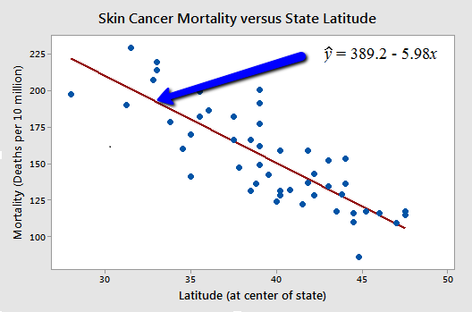
Is there a relationship between state latitude and skin cancer mortality? Certainly, since the estimated slope of the line, b1, is -5.98, not 0, there is a relationship between state latitude and skin cancer mortality in the sample of 49 data points. But, we want to know if there is a relationship between the population of all of the latitudes and skin cancer mortality rates. That is, we want to know if the population slope β₁ is unlikely to be 0.

An α-level hypothesis test for the slope parameter β₁

We follow standard hypothesis test procedures in conducting a hypothesis test for the slope β₁. First, we specify the null and alternative hypotheses:

Null hypothesis H₀ : β₁ = some number β
Alternative hypothesis H_A : β₁ ≠ some number β

The phrase "some number β" means that you can test whether or not the population slope takes on any value. Most often, however, we are interested in testing whether β₁ is 0. By default, statistical software conducts the hypothesis test with null hypothesis, β₁ is equal to 0, and alternative hypothesis, β₁ is not equal to 0. However, we can test values other than 0 and the alternative hypothesis can also state that β₁ is less than (<) some number β or greater than (>) some number β.

Second, we calculate the value of the test statistic using the following formula:

\[t^*=\frac{b_1-\beta}{\left(\frac{\sqrt{MSE}}{\sqrt{\sum(x_i-\bar{x})^2}} \right)}=\frac{b_1-\beta}{se(b_1)}\]

Third, we use the resulting test statistic to calculate the P-value. As always, the P-value is the answer to the question "how likely is it that we’d get a test statistic t* as extreme as we did if the null hypothesis were true?" The P-value is determined by referring to a t-distribution with n-2 degrees of freedom.

Finally, we make a decision:

• If the P-value is smaller than the significance level α, we reject the null hypothesis in favor of the alternative. We conclude "there is sufficient evidence at the α level to conclude that there is a linear relationship in the population between the predictor x and response y."
• If the P-value is larger than the significance level α, we fail to reject the null hypothesis. We conclude "there is not enough evidence at the α level to conclude that there is a linear relationship in the population between the predictor x and response y."

Drawing conclusions about the slope parameter β₁ using statistical software

Let's see how we can use statistical software to calculate conduct a hypothesis test for the slope β₁. Minitab's regression analysis output for our skin cancer mortality and latitude example appears below. The output for other software will be similar.

The line pertaining to the latitude predictor, Lat, in the summary table of predictors has been bolded. It tells us that the estimated slope coefficient b₁, under the column labeled Coef, is -5.9776. The estimated standard error of b₁, denoted se(b₁), in the column labeled SE Coef for "standard error of the coefficient," is 0.5984.

By default, the test statistic is calculated assuming the user wants to test that the slope is 0. Divide the estimated coefficient -5.9776 by the estimated standard error 0.5984 to obtain a test statistic T = -9.99.

By default, the P-value is calculated assuming the alternative hypothesis is a "two-tailed, not-equal-to" hypothesis. Calculate the probability that a t-random variable with n–2 = 47 degrees of freedom would be larger than 9.99 to get the probability in the upper tail. Then multiply this probability by 2 to get the two-tailed P-value, P = 0.000 (to three decimal places). In other words, the P-value is less than 0.001. (Note we multiply the probability by 2 since this is a two-tailed test. See this video for the reason why.)

Because the P-value is so small (less than 0.001), we can reject the null hypothesis and conclude that β₁ does not equal 0. There is sufficient evidence, at the α = 0.05 level, to conclude that there is a linear relationship in the population between skin cancer mortality and latitude.

Software Note. The P-value in statistical software regression analysis output is always calculated assuming the alternative hypothesis is testing the two-tailed β₁ ≠ 0. If your alternative hypothesis is the one-tailed β₁ < 0 or β₁ > 0, you have to divide the P-value that the software reports in the summary table of predictors by 2. (However, be careful if the test statistic is negative for an upper-tailed test or positive for a lower-tail test, in which case you have to divide by 2 and then subtract from 1. Draw a picture of an appropriately shaded density curve if you're not sure why.)

Six possible outcomes concerning slope β₁

There are six possible outcomes whenever we test whether there is a linear relationship between the predictor x and the response y, that is, whenever we test the null hypothesis H₀ : β₁ = 0 against the alternative hypothesis H_A : β₁ ≠ 0.

When we don't reject the null hypothesis H₀ : β₁ = 0, any of the following three realities are possible:

1. We committed a Type II error. That is, in reality β₁ ≠ 0 and our sample data just didn't provide enough evidence to conclude that β₁ ≠ 0.
2. There really is not much of a linear relationship between x and y.
3. There is a relationship between x and y — it is just not linear.

When we do reject the null hypothesis H₀ : β₁ = 0 in favor of the alternative hypothesis H_A : β₁ ≠ 0, any of the following three realities are possible:

1. We committed a Type I error. That is, in reality β₁ = 0, but we have an unusual sample that suggests that β₁ ≠ 0.
2. The relationship between x and y is indeed linear.
3. A linear function fits the data okay, but a curved ("curvilinear") function would fit the data even better.

(1-α)100% t-interval for the slope parameter β₁

The formula for the confidence interval for β₁, in words, is:

Sample estimate ± (t-multiplier × standard error)

and, in notation, is:

\[b_1 \pm t_{(\alpha/2, n-2)}\times \left( \frac{\sqrt{MSE}}{\sqrt{\sum(x_i-\bar{x})^2}} \right)\]

The resulting confidence interval not only gives us a range of values that is likely to contain the true unknown value β₁. It also allows us to answer the research question "is the predictor x linearly related to the response y?" If the confidence interval for β₁ contains 0, then we conclude that there is no evidence of a linear relationship between the predictor x and the response y in the population. On the other hand, if the confidence interval for β₁ does not contain 0, then we conclude that there is evidence of a linear relationship between the predictor x and the response y in the population.

It's easy to calculate a 95% confidence interval for β₁ using the information in the software output. You just need to find the t-multiplier, either from a table or by using statistical software. In this case it is t(0.025, 47) = 2.0117. Then, the 95% confidence interval for β₁ is -5.9776 ± 2.0117(0.5984) or (-7.2, -4.8). [Alternatively, some statistical software will display the interval directly.]

We can be 95% confident that the population slope is between -7.2 and -4.8. That is, we can be 95% confident that for every additional one-degree increase in latitude, the mean skin cancer mortality rate decreases between 4.8 and 7.2 deaths per 10 million people.

Factors affecting the width of a confidence interval for β₁

Recall that, in general, we want our confidence intervals to be as narrow as possible to be the most informative. If we know what factors affect the length of a confidence interval for the slope β₁, we can control them to ensure that we obtain a narrow interval. The factors can be easily determined by studying the formula for the confidence interval:

\[b_1 \pm t_{\alpha/2, n-2}\times \left(\frac{\sqrt{MSE}}{\sqrt{\sum(x_i-\bar{x})^2}} \right) \]

First, subtracting the lower endpoint of the interval from the upper endpoint of the interval, we determine that the width of the interval is:

\[\text{Width }=2 \times t_{\alpha/2, n-2}\times \left(\frac{\sqrt{MSE}}{\sqrt{\sum(x_i-\bar{x})^2}} \right)\]

So, how can we affect the width of our resulting interval for β₁?

• As the confidence level decreases, the width of the interval decreases. Therefore, if we decrease our confidence level, we decrease the width of our interval. Clearly, we don't want to decrease the confidence level too much. Typically, confidence levels are never set below 90%.
• As MSE decreases, the width of the interval decreases. The value of MSE depends on only two factors — how much the responses vary naturally around the estimated regression line, and how well your regression function (line) fits the data. Clearly, you can't control the first factor all that much other than to ensure that you are not adding any unnecessary error in your measurement process. Throughout this course, we'll learn ways to make sure that the regression function fits the data as well as it can.
• The more spread out the predictor x values, the narrower the interval. The quantity \(\sum(x_i-\bar{x})^2\) in the denominator summarizes the spread of the predictor x values. The more spread out the predictor values, the larger the denominator, and hence the narrower the interval. Therefore, we can decrease the width our interval by ensuring that our predictor values are sufficiently spread out.
• As the sample size increases, the width of the interval decreases. The sample size plays a role in two ways. First, recall that the t-multiplier depends on the sample size through n-2. Therefore, as the sample size increases, the t-multiplier decreases, the length of the interval decreases. Second, the denominator \(\sum(x_i-\bar{x})^2\) also depends on n. The larger the sample size, the more terms you add to this sum, the larger the denominator, the narrower the interval. Therefore, in general, you can ensure that your interval is narrow by having a large enough sample.

An α-level hypothesis test for intercept parameter β₀

Conducting hypothesis tests and calculating confidence intervals for the intercept parameter β₀ is not done as often as it is for the slope parameter β₁. The reason for this becomes clear upon reviewing the meaning of β₀. The intercept parameter β₀ is the mean of the responses at x = 0. If x = 0 is meaningless, as it would be, for example, if your predictor variable was height, then β₀ is not meaningful. For the sake of completeness, we present the methods here for those rare situations in which β₀ is meaningful.

To conduct a hypothesis test for the intercept parameter β₀ we again follow standard hypothesis test procedures. First, we specify the null and alternative hypotheses:

Null hypothesis H₀ : β₀ = some number β
Alternative hypothesis H_A: β₀ ≠ some number β

The phrase "some number β" means that you can test whether or not the population intercept takes on any value. By default, statistical software conducts the hypothesis test for testing whether or not β₀ is 0. But, the alternative hypothesis can also state that β₀ is less than (<) some number β or greater than (>) some number β.

Second, we calculate the value of the test statistic using the following formula:

\[t^*=\frac{b_0-\beta}{\sqrt{MSE} \sqrt{\frac{1}{n}+\frac{\bar{x}^2}{\sum(x_i-\bar{x})^2}}}=\frac{b_0-\beta}{se(b_0)}\]

Third, we use the resulting test statistic to calculate the P-value. Again, the P-value is the answer to the question "how likely is it that we’d get a test statistic t* as extreme as we did if the null hypothesis were true?" The P-value is determined by referring to a t-distribution with n-2 degrees of freedom.

Finally, we make a decision. If the P-value is smaller than the significance level α, we reject the null hypothesis in favor of the alternative. If we conduct a "two-tailed, not-equal-to-0" test, we conclude "there is sufficient evidence at the α level to conclude that the mean of the responses is not 0 when x = 0." If the P-value is larger than the significance level α, we fail to reject the null hypothesis.

Drawing conclusions about intercept parameter β₀ using statistical software

Let's see how we can use statistical software to conduct a hypothesis test for the intercept β₀. Statistical software regression analysis output for our skin cancer mortality and latitude example appears below. The work involved is very similar to that for the slope β₁.

The line pertaining to the intercept is labeled Constant (but in other software may be labeled Intercept). It tells us that the estimated intercept coefficient b₀, under the column labeled Coef, is 389.19. The estimated standard error of b₀, denoted se(b₀), in the column labeled SE Coef is 23.81.

By default, the test statistic is calculated assuming the user wants to test that the mean response is 0 when x = 0. Note that this is an ill-advised test here, because the predictor values in the sample do not include a latitude of 0. That is, such a test involves extrapolating outside the scope of the model. Nonetheless, for the sake of illustration, let's proceed assuming that it is an okay thing to do.

Dividing the estimated coefficient 389.19 by the estimated standard error 23.81, the test statistic T is 16.34. By default, the P-value is calculated assuming the alternative hypothesis is a "two-tailed, not-equal-to-0" hypothesis. The probability that a t random variable with n-2 = 47 degrees of freedom would be larger than 16.34, and multiplying that probability by 2, the P-value is P = 0.000 (to three decimal places). That is, the P-value is less than 0.001.

Because the P-value is so small (less than 0.001), we can reject the null hypothesis and conclude that β₀ does not equal 0 when x = 0. There is sufficient evidence, at the α = 0.05 level, to conclude that the mean mortality rate at a latitude of 0 degrees North is not 0. (Again, note that we have to extrapolate beyond the scope of the model in order to arrive at this conclusion, which in general is not advisable.)

(1-α)100% t-interval for intercept parameter β₀

The formula for the confidence interval for β₀, in words, is:

Sample estimate ± (t-multiplier × standard error)

and, in notation, is:

\[b_0 \pm t_{\alpha/2, n-2} \times \sqrt{MSE} \sqrt{\frac{1}{n}+\frac{\bar{x}^2}{\sum(x_i-\bar{x})^2}}\]

The resulting confidence interval gives us a range of values that is likely to contain the true unknown value β₀. The factors affecting the length of a confidence interval for β₀ are identical to the factors affecting the length of a confidence interval for β₁.

Proceed as previously described to calculate a 95% confidence interval for β₀. Find the t-multiplier using a table or statistical software. Again, it is t(0.025, 47) = 2.0117. Then, the 95% confidence interval for β₀ is 389.19 ± 2.0117(23.81) = (341.3, 437.1). [Alternatively, if possible, use statistical software to display the interval directly.] We can be 95% confident that the population intercept is between 341.3 and 437.1. That is, we can be 95% confident that the mean mortality rate at a latitude of 0 degrees North is between 341.3 and 437.1 deaths per 10 million people. (Again, it is probably not a good idea to make this claim because of the severe extrapolation involved.)

Statistical inference conditions

We've made no mention yet of the conditions that must be true in order for it to be okay to use the above hypothesis testing procedures and confidence interval formulas for β₀ and β₁. In short, the "LINE" assumptions we discussed earlier — linearity, independence, normality and equal variance — must hold. It is not a big deal if the error terms (and thus responses) are only approximately normal. If you have a large sample, then the error terms can even deviate somewhat far from normality.

Regression through the origin

In rare circumstances it may make sense to consider a simple linear regression model in which the intercept, β₀, is assumed to be exactly 0. For example, suppose we have data on the number of items produced per hour along with the number of rejects in each of those time spans. If we have a period where no items were produced, then there are obviously 0 rejects. Such a situation may indicate deleting β₀ from the model since β₀ reflects the amount of the response (in this case, the number of rejects) when the predictor is assumed to be 0 (in this case, the number of items produced). Thus, the model to estimate becomes

\[\begin{equation*} y_{i}=\beta_{1}x_{i}+\epsilon_{i},\end{equation*}\]

which is called a regression through the origin (or RTO) model. The estimate for \(\beta_{1}\)when using the regression through the origin model is:

\[\hat{\beta}_{\textrm{RTO}}=\frac{\sum_{i=1}^{n}x_{i}y_{i}}{\sum_{i=1}^{n}x_{i}^{2}}.\]

Thus, the estimated regression equation is

\[\begin{equation*} \hat{y}_{i}=\hat{\beta}_{\textrm{RTO}}x_{i}\end{equation*}.\]

Note that this formula no longer centers (or "adjusts") the \(x_{i}\)'s and \(y_{i}\)'s by their sample means (compare this estimate for \(\hat{\beta}_{1}\) to that of the estimate found for the simple linear regression model). Since there is no intercept, there is no correction factor and no adjustment for the mean (i.e., the regression line can only pivot about the point (0,0)).

Generally, a regression through the origin is not recommended due to the following:

1. Removal of \(\beta_{0}\) is a strong assumption which forces the line to go through the point (0,0). Imposing this restriction does not give ordinary least squares as much flexibility in finding the line of best fit for the data.
2. In a simple linear regression model, \(\sum_{i=1}^{n}(y_{i}-\hat{y}_i)=\sum_{i=1}^{n}e_{i}=0\). However, in regression through the origin, generally \(\sum_{i=1}^{n}e_{i}\neq 0\). Because of this, the SSE could actually be larger than the SSTO, thus resulting in \(r^{2}<0\).
3. Since \(r^{2}\) can be negative, the usual interpretation of this value as a measure of the strength of the linear component in the simple linear regression model cannot be used here.

If you strongly believe that a regression through the origin model is appropriate for your situation, then statistical testing can help justify your decision. However, if no data has been collected near \(x=0\), then forcing the regression line through the origin is likely to make for a worse-fitting model. So again, this model is not usually recommended unless there is a strong belief that it is appropriate.

Statistical software generally includes an option to fit a "regression through the origin" model.