3.8 - The Lack of Fit F-test When There Are Replicates
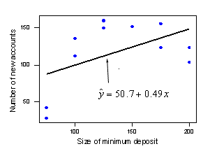
We're almost there! We just need to determine an objective way of deciding when too much of the error in our prediction is due to lack of model fit. That's where the lack of fit F-test comes into play. Let's return to the first checking account example, (newaccounts.txt):

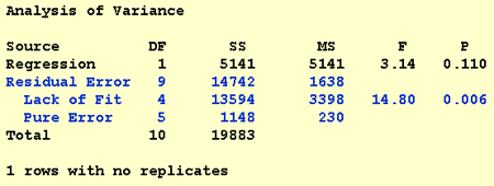
Jumping ahead to the punchline, here's statistical software output for the lack of fit F-test for this data set:

As you can see, the lack of fit output appears as a portion of the analysis of variance table. In the Sum of Squares ("SS") column, we see — as we previously calculated — that SSLF = 13594 and SSPE = 1148 sum to SSE = 14742. We also see in the Degrees of Freedom ("DF") column that — since there are n = 11 data points and c = 6 distinct x values (75, 100, 125, 150, 175, and 200) — the lack of fit degrees of freedom c - 2 = 4 and the pure error degrees of freedom is n - c = 5 sum to the error degrees of freedom n - 2 = 9.
Just as is done for the sums of squares in the basic analysis of variance table, the lack of fit sum of squares and the error sum of squares are used to calculate "mean squares." They are even calculated similarly, namely by dividing the sum of squares by its associated degrees of freedom. Here are the formal definitions of the mean squares:
- The "lack of fit mean square" is \(MSLF=\frac{\sum\sum(\bar{y}_i-\hat{y}_{ij})^2}{c-2}=\frac{SSLF}{c-2}\)
- The "pure error mean square" is \(MSPE=\frac{\sum\sum(y_{ij}-\bar{y}_{i})^2}{n-c}=\frac{SSPE}{n-c}\)
In the Mean Squares ("MS") column in the software output above, we see that the lack of fit mean square MSLF is 13594 divided by 4, or 3398. The pure error mean square MSPE is 1148 divided by 5, or 230.
You might notice that the lack of fit F-statistic is calculated by dividing the lack of fit mean square (MSLF = 3398) by the pure error mean square (MSPE = 230) to get 14.80. How do we know that this F-statistic helps us in testing the hypotheses:
- H0: The relationship assumed in the model is reasonable, i.e., there is no lack of fit.
- HA: The relationship assumed in the model is not reasonable, i.e., there is lack of fit.
The answer lies in the "expected mean squares." In our sample of n = 11 newly opened checking accounts, we obtained MSLF = 3398. If we had taken a different random sample of size n = 11, we would have obtained a different value for MSLF. Theory tells us that the average of all of the possible MSLF values we could obtain is:
\[E(MSLF) =\sigma^2+\frac{\sum n_i(\mu_i-(\beta_0+\beta_1X_i))^2}{c-2}\]
That is, we should expect MSLF, on average, to equal the above quantity — σ2 plus another messy-looking term. Think about that messy term. If the null hypothesis is true, i.e., if the relationship between the predictor x and the response y is linear, then μi equals β0 + β1Xi and the messy term becomes 0 and goes away. That is, if there is no lack of fit, we should expect the lack of fit mean square MSLF to equal σ2.
What should we expect MSPE to equal? Theory tells us it should, on average, always equal σ2:
\[E(MSPE) =\sigma^2\]
Aha — there we go! The logic behind the calculation of the F-statistic is now clear:
- If there is a linear relationship between x and y, then μi = β0 + β1Xi. That is, there is no lack of fit in the simple linear regression model. We would expect the ratio MSLF/MSPE to be close to 1.
- If there is not a linear relationship between x and y, then μi ≠ β0 + β1Xi. That is, there is lack of fit in the simple linear regression model. We would expect the ratio MSLF/MSPE to be large, i.e., a value greater than 1.
So, to conduct the lack of fit test, we calculate the value of the F-statistic:
\[F^*=\frac{MSLF}{MSPE}\]
and determine if it is large. To decide if it is large, we compare the F*-statistic to an F-distribution with c - 2 numerator degrees of freedom and n - c denominator degrees of freedom.
In summary
We follow standard hypothesis test procedures in conducting the lack of fit F-test. First, we specify the null and alternative hypotheses:
- H0: The relationship assumed in the model is reasonable, i.e., there is no lack of fit in the model μi = β0 + β1Xi.
- HA: The relationship assumed in the model is not reasonable, i.e., there is lack of fit in the model μi = β0 + β1Xi.
Second, we calculate the value of the F-statistic:
\[F^*=\frac{MSLF}{MSPE}\]
To do so, we complete the analysis of variance table using the following formulas.
|
Source of Variation
|
DF
|
SS
|
MS
|
F
|
|
Regression
|
1
|
\(SSR=\sum_{i=1}^{c}\sum_{j=1}^{n_i}(\hat{y}_{ij}-\bar{y})^2\)
|
\[MSR=\frac{SSR}{1}\]
|
\[F=\frac{MSR}{MSE}\]
|
|
Residual error
|
n - 2
|
\(SSE=\sum_{i=1}^{c}\sum_{j=1}^{n_i}(y_{ij}-\hat{y}_{ij})^2\)
|
\[MSE=\frac{SSE}{n-2}\]
|
|
|
Lack of Fit
|
c - 2
|
\(SSLF=\sum_{i=1}^{c}\sum_{j=1}^{n_i}(\bar{y}_{i}-\hat{y}_{ij})^2\)
|
\[MSLF=\frac{SSLF}{c-2}\]
|
\[F^*=\frac{MSLF}{MSPE}\]
|
| Pure error |
n - c
|
\(SSPE=\sum_{i=1}^{c}\sum_{j=1}^{n_i}(y_{ij}-\bar{y}_{i})^2\)
|
\[MSPE=\frac{SSPE}{n-c}\]
|
|
|
Total
|
n - 1
|
\(SSTO=\sum_{i=1}^{c}\sum_{j=1}^{n_i}(y_{ij}-\bar{y})^2\)
|
|
|
In reality, we let statistical software determine the analysis of variance table for us.
Third, we use the resulting F*-statistic to calculate the P-value. As always, the P-value is the answer to the question "how likely is it that we’d get an F*-statistic as extreme as we did if the null hypothesis were true?" The P-value is determined by referring to an F-distribution with c - 2 numerator degrees of freedom and n - c denominator degrees of freedom.
Finally, we make a decision:
- If the P-value is smaller than the significance level α, we reject the null hypothesis in favor of the alternative. We conclude "there is sufficient evidence at the α level to conclude that there is lack of fit in the simple linear regression model."
- If the P-value is larger than the significance level α, we fail to reject the null hypothesis. We conclude "there is not enough evidence at the α level to conclude that there is lack of fit in the simple linear regression model."
For our checking account example the F*-statistic is 14.80 and the P-value is 0.006. The P-value is smaller than the significance level α = 0.05 — we reject the null hypothesis in favor of the alternative. There is sufficient evidence at the α = 0.05 level to conclude that there is lack of fit in the simple linear regression model. In light of the scatter plot, the lack of fit test provides the answer we expected.
Formal lack of fit testing can also be performed in the multiple regression setting that we consider later in the course. However, the ability to achieve replicates can be more difficult as more predictors are added to the model.

