In this section, we are concerned with the confidence interval, called a "t-interval," for the mean response μ_Y when the predictor value is x_h. Let's jump right in and learn the formula for the confidence interval. The general formula in words is as always:

Sample estimate ± (t-multiplier × standard error)

and the formula in notation is:

\[\hat{y}_h \pm t_{(\alpha/2, n-2)} \times \sqrt{MSE \times \left( \frac{1}{n} + \frac{(x_h-\bar{x})^2}{\sum(x_i-\bar{x})^2}\right)}\]

where:

• \(\hat{y}_h\) is the "fitted value" or "predicted value" of the response when the predictor is \(x_h\)
• \(t_{(\alpha/2, n-2)}\) is the "t-multiplier." Note that the t-multiplier has n-2 (not n-1) degrees of freedom, because the confidence interval uses the mean square error (MSE) whose denominator is n-2.
• \(\sqrt{MSE \times \left( \frac{1}{n} + \frac{(x_h-\bar{x})^2}{\sum(x_i-\bar{x})^2}\right)}\) is the "standard error of the fit," which depends on the mean square error (MSE), the sample size (n), how far in squared units the predictor value \(x_h\) is from the average of the predictor values \(\bar{x}\), or \((x_h-\bar{x})^2\) , and the sum of the squared distances of the predictor values \(x_i\) from the average of the predictor values \(\bar{x}\), or \(\sum(x_i-\bar{x})^2\).

Fortunately, we won't have to use the formula to calculate the confidence interval, since statistical software will do the dirty work for us. Here is some output for our example with "skin cancer mortality" as the response and "latitude" as the predictor (skincancer.txt):

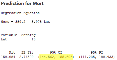
Here's what the output tells us:

• Variable setting: the value x_h (40 degrees north) for which we requested the confidence interval for µ_Y.
• The predicted value \(\hat{y}_h\), ("Fit" = 150.084) and the standard error of the fit ("SE Fit" = 2.74500).
• 95% CI: the 95% confidence interval. We can be 95% confident that the average skin cancer mortality rate of all locations at 40 degrees north is between 144.562 and 155.606 deaths per 10 million people.
• 95% PI: the 95% prediction interval for a new response (which we discuss in the next section).

Factors affecting the width of the t-interval for the mean response µ_Y

Why do we bother learning the formula for the confidence interval for µ_Y when we let statistical software calculate it for us anyway? As always, the formula is useful for investigating what factors affect the width of the confidence interval for µ_Y. Again, the formula is:

\[\hat{y}_h \pm t_{(\alpha/2, n-2)} \times \sqrt{MSE \times \left( \frac{1}{n} + \frac{(x_h-\bar{x})^2}{\sum(x_i-\bar{x})^2}\right)}\]

and therefore the width of the confidence interval for µ_Y is:

\[2 \times \left[t_{(\alpha/2, n-2)} \times \sqrt{MSE \times \left( \frac{1}{n} + \frac{(x_h-\bar{x})^2}{\sum(x_i-\bar{x})^2}\right)}\right]\]

So how can we affect the width of our resulting interval for µ_Y?

• As the mean square error (MSE) decreases, the width of the interval decreases. Since MSE is an estimate of how much the data vary naturally around the unknown population regression line, we have little control over MSE other than making sure that we make our measurements as carefully as possible. (We will return to this issue later in the course when we address "model selection.")
• As we decrease the confidence level, the t-multiplier decreases, and hence the width of the interval decreases. In practice, we wouldn't want to set the confidence level below 90%.
• As we increase the sample size n, the width of the interval decreases. We have complete control over the size of our sample — the only limitation beting our time and financial constraints.
• The more spread out the predictor values, the larger the quantity \(\sum(x_i-\bar{x})^2\) and hence the narrower the interval. In general, you should make sure your predictor values are not too clumped together but rather sufficiently spread out.
• The closer x_h is to the average of the sample's predictor values \(\bar{x}\), the smaller the quantity \((x_h-\bar{x})^2\), and hence the narrower the interval. If you know that you want to use your estimated regression equation to estimate µ_Y when the predictor's value is x_h, then you should be aware that the confidence interval will be narrower the closer x_h is to \(\bar{x}\).

Let's see this last claim in action for our example with "skin cancer mortality" as the response and "latitude" as the predictor:

The software output reports a 95% confidence interval for µ_Y for a latitude of 40 degrees north (first row) and 28 degrees north (second row). The average latitude of the 49 states in the data set is 39.533 degrees north. The output tells us:

• We can be 95% confident that the mean skin cancer mortality rate of all locations at 40 degrees north is between 144.6 and 155.6 deaths per 10 million people.
• And, we can be 95% confident that the mean skin cancer mortality rate of all locations at 28 degrees north is between 206.9 and 236.8 deaths per 10 million people.

The width of the 40 degree north interval (155.6 - 144.6 = 11 deaths) is shorter than the width of the 28 degree north interval (236.8 - 206.9 = 29.9 deaths), because 40 is much closer than 28 is to the sample mean 39.533. Note that some software is kind enough to warn us that 28 degrees north is far from the mean of the sample's predictor values.

When is it okay to use the formula for the confidence interval for µ_Y?

One thing we haven't discussed yet is when it is okay to use the formula for the confidence interval for µ_Y. It is okay:

• When x_h is a value within the range of the x values in the data set — that is, when x_h is a value within the "scope of the model." But, note that x_h does not have to be one of the actual x values in the data set.
• When the "LINE" conditions — linearity, independent errors, normal errors, equal error variances — are met. The formula works okay even if the error terms are only approximately normal. And, if you have a large sample, the error terms can even deviate substantially from normality.