In this section, we are concerned with the prediction interval for a new response y_new when the predictor's value is x_h. Again, let's just jump right in and learn the formula for the prediction interval. The general formula in words is as always:

Sample estimate ± (t-multiplier × standard error)

and the formula in notation is:

\[\hat{y}_h \pm t_{(\alpha/2, n-2)} \times \sqrt{MSE \left( 1+\frac{1}{n} + \frac{(x_h-\bar{x})^2}{\sum(x_i-\bar{x})^2}\right)}\]

where:

• \(\hat{y}_h\) is the "fitted value" or "predicted value" of the response when the predictor is \(x_h\)
• \(t_{(\alpha/2, n-2)}\) is the "t-multiplier." Note again that the t-multiplier has n-2 (not n-1) degrees of freedom, because the prediction interval uses the mean square error (MSE) whose denominator is n-2.
• \(\sqrt{MSE \times \left( 1+\frac{1}{n} + \frac{(x_h-\bar{x})^2}{\sum(x_i-\bar{x})^2}\right)}\) is the "standard error of the prediction," which is very similar to the "standard error of the fit" when estimating µ_Y. The standard error of the prediction just has an extra MSE term added that the standard error of the fit does not. (More on this a bit later.)

Again, we won't use the formula to calculate our prediction intervals. We'll let statistical software do the calculation for us. Let's look at the prediction interval for our example with "skin cancer mortality" as the response and "latitude" as the predictor (skincancer.txt):

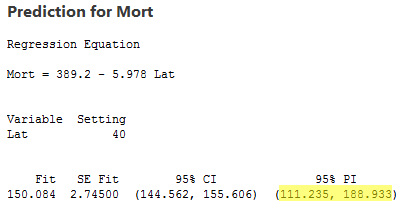
The output reports the 95% prediction interval for an individual location at 40 degrees north. We can be 95% confident that the skin cancer mortality rate at an individual location at 40 degrees north will be between 111.235 and 188.933 deaths per 10 million people.

When is it okay to use the prediction interval for y_new formula?

The requirements are similar to, but a little more restrictive than, those for the confidence interval. It is okay:

• When x_h is a value within the scope of the model. Again, x_h does not have to be one of the actual x values in the data set.
• When the "LINE" conditions — linearity, independent errors, normal errors, equal error variances — are met. Unlike the case for the formula for the confidence interval, the formula for the prediction interval depends strongly on the condition that the error terms are normally distributed.

Understanding the difference in the two formulas

In our discussion of the confidence interval for µ_Y, we used the formula to investigate what factors affect the width of the confidence interval. There's no need to do it again. Because the formulas are so similar, it turns out that the factors affecting the width of the prediction interval are identical to the factors affecting the width of the confidence interval.

Let's instead investigate the formula for the prediction interval for y_new:

\[\hat{y}_h \pm t_{(\alpha/2, n-2)} \times \sqrt{MSE \times \left( 1+\frac{1}{n} + \frac{(x_h-\bar{x})^2}{\sum(x_i-\bar{x})^2}\right)}\]

to see how it compares to the formula for the confidence interval for µ_Y:

\[\hat{y}_h \pm t_{(\alpha/2, n-2)} \times \sqrt{MSE \left(\frac{1}{n} + \frac{(x_h-\bar{x})^2}{\sum(x_i-\bar{x})^2}\right)}\]

Observe that the only difference in the formulas is that the standard error of the prediction for y_new has an extra MSE term in it that the standard error of the fit for µ_Y does not.

Let's try to understand the prediction interval to see what causes the extra MSE term. In doing so, let's start with an easier problem first. Think about how we could predict a new response y_new at a particular x_h if the mean of the responses µ_Y at x_h were known. That is, suppose it were known that the mean skin cancer mortality at x_h = 40^o N is 150 deaths per million (with variance 400)? What is the predicted skin cancer mortality in Columbus, Ohio?

Because µ_Y = 150 and σ² = 400 are known, we can take advantage of the "empirical rule," which states among other things that 95% of the measurements of normally distributed data are within 2 standard deviations of the mean. That is, it says that 95% of the measurements are in the interval sandwiched by:

µ_Y - 2σ and µ_Y + 2σ.

Applying the 95% rule to our example with µ_Y = 150 and σ = 20:

95% of the skin cancer mortality rates of locations at 40 degrees north latitude are in the interval sandwiched by:

150 - 2(20) = 110 and 150 + 2(20) = 190.

That is, if someone wanted to know the skin cancer mortality rate for a location at 40 degrees north, our best guess would be somewhere between 110 and 190 deaths per 10 million. The problem is that our calculation used µ_Y and σ, population values that we would typically not know. Reality sets in:

• The mean µ_Y is typically not known. The logical thing to do is estimate it with the predicted response \(\hat{y}\). The cost of using \(\hat{y}\) to estimate µ_Y is the variance of \(\hat{y}\). That is, different samples would yield different predictions \(\hat{y}\), and so we have to take into account this variance of \(\hat{y}\).
• The variance σ² is typically not known. The logical thing to do is to estimate it with MSE.

Because we have to estimate these unknown quantities, the variation in the prediction of a new response depends on two components:

1. the variation due to estimating the mean µ_Y with \(\hat{y}_h\) , which we denote "\(\sigma^2(\hat{Y}_h)\)." (Note that the estimate of this quantity is just the standard error of the fit that appears in the confidence interval formula.)
2. the variation in the responses y, which we denote as "\(\sigma^2\)." (Note that quantity is estimated, as usual, with the mean square error MSE.)

Adding the two variance components, we get:

\[\sigma^2+\sigma^2(\hat{Y}_h)\]

which is estimated by:

\[MSE+MSE \left[  \frac{1}{n} + \frac{(x_h-\bar{x})^2}{\sum_{i=1}^{n}(x_i-\bar{x})^2} \right] =MSE\left[ 1+\frac{1}{n} + \frac{(x_h-\bar{x})^2}{\sum_{i=1}^{n}(x_i-\bar{x})^2}  \right] \]

Do you recognize this quantity? It's just the variance of the prediction that appears in the formula for the prediction interval y_new!

Let's compare the two intervals again:

Confidence interval for µ_Y:   \[\hat{y}_h \pm t_{(\alpha/2, n-2)} \times \sqrt{MSE \times \left( \frac{1}{n} + \frac{(x_h-\bar{x})^2}{\sum(x_i-\bar{x})^2}\right)}\]

Prediction interval for y_new:   \[\hat{y}_h \pm t_{(\alpha/2, n-2)} \times \sqrt{MSE \left( 1+\frac{1}{n} + \frac{(x_h-\bar{x})^2}{\sum(x_i-\bar{x})^2}\right)}\]

What's the practical implications of the difference in the two formulas?

• Because the prediction interval has the extra MSE term, a (1-α)100% confidence interval for µ_Y at x_h will always be narrower than the corresponding (1-α)100% prediction interval for y_new at x_h.
• By calculating the interval at the sample's mean of the predictor values (x_h = \(\bar{x}\)) and increasing the sample size n, the confidence interval's standard error can approach 0. Because the prediction interval has the extra MSE term, the prediction interval's standard error cannot get close to 0.

The first implication is seen most easily by studying the following plot for our skin cancer mortality example:

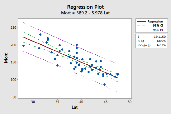
Observe that the prediction interval (in purple) is always wider than the confidence interval (in green). Furthermore, both intervals are narrowest at the mean of the predictor values (about 39.5).