Let's jump in and take a look at some "real-life" examples in which a multiple linear regression model is used. Make sure you notice, in each case, that the model has more than one predictor. You might also try to pay attention to the similarities and differences among the examples and their resulting models. Most of all, don't worry about mastering all of the details now. In the upcoming lessons, we will re-visit similar examples in greater detail. For now, my hope is that these examples leave you with an appreciation of the richness of multiple regression.

Are a person's brain size and body size predictive of his or her intelligence?

Interested in answering the above research question, some researchers (Willerman, et al, 1991) collected the following data (iqsize.txt) on a sample of n = 38 college students:

• Response (y): Performance IQ scores (PIQ) from the revised Wechsler Adult Intelligence Scale. This variable served as the investigator's measure of the individual's intelligence.
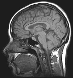
• Potential predictor (x₁): Brain size based on the count obtained from MRI scans (given as count/10,000).
• Potential predictor (x₂): Height in inches.
• Potential predictor (x₃): Weight in pounds.

As always, the first thing we should want to do when presented with a set of data is to plot it. And, of course, plotting the data is a little more challenging in the multiple regression setting, as there is one scatter plot for each pair of variables. Not only do we have to consider the relationship between the response and each of the predictors, we also have to consider how the predictors are related among each other.

A common way of investigating the relationships among all of the variables is by way of a "scatter plot matrix." Basically, a scatter plot matrix contains a scatter plot of each pair of variables arranged in an orderly array. Here's what one version of a scatter plot matrix looks like for our brain and body size example:  

For each scatter plot in the matrix, the variable on the y-axis appears at the left end of the plot's row and the variable on the x-axis appears at the bottom of the plot's column. Try to identify the variables on the y-axis and x-axis in each of the six scatter plots appearing in the matrix. You can check your understanding by rolling your mouse over each scatter plot appearing in the above matrix.

Incidentally, in case you are wondering, the tick marks on each of the axes are located at 25% and 75% of the data range from the minimum. That is:

• the first tick = ((maximum - minimum) * 0.25) + minimum
• the second tick = ((maximum - minimum) * 0.75) + minimum

Sometimes software packages use a different scheme in labeling the scatter plot matrix. For each plot in the following scatter plot matrix, the variable on the y-axis appears at the right end of the plot's row and the variable on the x-axis appears at the top of the plot's column. Again, you can roll your mouse over each scatter plot appearing in the matrix to make sure you understand this different labeling scheme:

Now, what does a scatter plot matrix tell us? Of course, one use of the plots is simple data checking. Are there any egregiously erroneous data errors? The scatter plots also illustrate the "marginal relationships" between each pair of variables without regard to the other variables. For example, it appears that brain size is the best single predictor of PIQ, but none of the relationships are particularly strong. In multiple linear regression, the challenge is to see how the response y relates to all three predictors simultaneously.

We always start a regression analysis by formulating a model for our data. One possible multiple linear regression model with three quantitative predictors for our brain and body size example is:

\[y_i=(\beta_0+\beta_1x_{i1}+\beta_2x_{i2}+\beta_3x_{i3})+\epsilon_i\] 

where:

• y_i is the intelligence (PIQ) of student i
• x_i1 is the brain size (MRI) of student i
• x_i2 is the height (Height) of student i
• x_i3 is the weight (Weight) of student i

and the independent error terms ε_i follow a normal distribution with mean 0 and equal variance σ².

A couple of things to note about this model:

• Because we have more than one predictor (x) variable, we use slightly modified notation. The x-variables (e.g., x_i1, x_i2, and x_i3) are now subscripted with a 1, 2, and 3 as a way of keeping track of the three different quantitative variables. We also subscript the slope parameters with the corresponding numbers (e.g., β₁ β₂ and β₃).
• The "LINE" conditions must still hold for the multiple linear regression model. The linear part comes from the formulated regression function — it is, what we say, "linear in the parameters." This simply means that each beta coefficient multiplies a predictor variable or a transformation of one or more predictor variables. We'll see in Lesson 7 that this means that, for example, the model, \(y=\beta_0+\beta_1x+\beta_2x^2+\epsilon\), is a multiple linear regression model even though it represents a curved relationship between \(y\) and \(x\).

Of course, our interest in performing a regression analysis is almost always to answer some sort of research question. Can you think of some research questions that the researchers might want to answer here? How about the following set of questions? What procedure would you use to answer each research question? (Do the procedures that appear in parentheses seem reasonable?)

• Which, if any, predictors — brain size, height, or weight — explain some of the variation in intelligence scores? (Conduct hypothesis tests for individually testing whether each slope parameter could be 0.)
• What is the effect of brain size on PIQ, after taking into account height and weight? (Calculate and interpret a confidence interval for the brain size slope parameter.)
• What is the PIQ of an individual with a given brain size, height, and weight? (Calculate and interpret a prediction interval for the response.)

Let's take a look at statistical software output for the multiple regression model we formulated above:

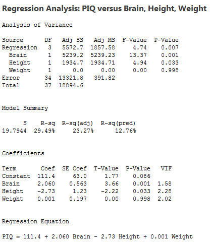
My hope is that you immediately observe that much of the output looks the same as before! The only substantial differences are:

• More predictors appear in the estimated regression equation and therefore also in the column labeled "Term" in the table of estimates.
• There is an additional row for each predictor term in the Analysis of Variance Table. The label "Adj SS" indicates that these represent the increase in regression sums of squares for each term relative to a model that contains all of the other terms in the model (so-called Adjusted or Type III sums of squares). It is usually possible to instead use Sequential or Type I sums of squares, which represent the increase in regression sums of squares when a term is added to a model that contains only the terms listed before it in the ANOVA table.

We'll learn more about these differences later, but let's focus now on what you already know. The output tells us that:

• The R² value is 29.49%. This tells us that 29.49% of the variation in intelligence, as quantified by PIQ, is reduced by taking into account brain size, height and weight.
• The Adjusted R² value — denoted "R-sq(adj)" — is 23.27%. When considering different multiple linear regression models for PIQ, we could use this value to help compare the models.
• The P-values for the t-tests appearing in the table of estimates suggest that the slope parameters for Brain (P = 0.001) and Height (P = 0.033) are significantly different from 0, while the slope parameter for Weight (P = 0.998) is not.
• The P-value for the analysis of variance F-test (P = 0.007) suggests that the model containing Brain, Height and Weight is more useful in predicting intelligence than not taking into account the three predictors. (Note that this does not tell us that the model with the three predictors is the best model!)

So, we already have a pretty good start on this multiple linear regression stuff. Let's take a look at another example.