Example 1: Pastry Sweetness Data

A designed experiment is done to assess how moisture content and sweetness of a pastry product affect a taster’s rating of the product (pastry.txt). In a designed experiment, the eight possible combinations of four moisture levels and two sweetness levels are studied. Two pastries are prepared and rated for each of the eight combinations, so the total sample size is n = 16. The y-variable is the rating of the pastry. The two x-variables are moisture and sweetness. The values (and sample sizes) of the x-variables were designed so that the x-variables were not correlated.

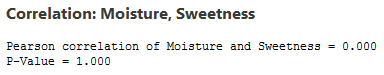
A plot of moisture versus sweetness (the two x-variables) is as follows:

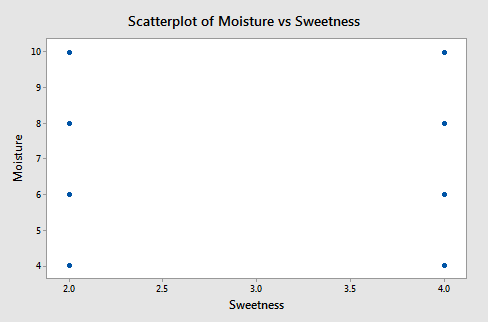
Notice that the points are on a rectangular grid so the correlation between the two variables is 0. (Please Note: we are not able to see that actually there are 2 observations at each location of the grid!)

The following figure shows how the two x-variables affect the pastry rating.

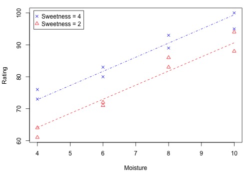
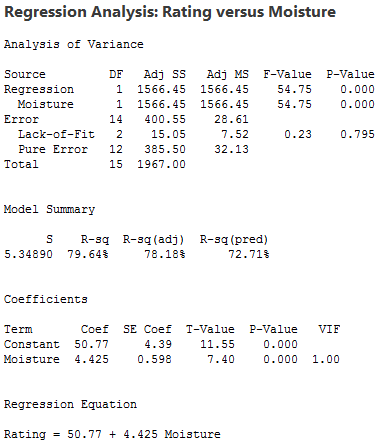
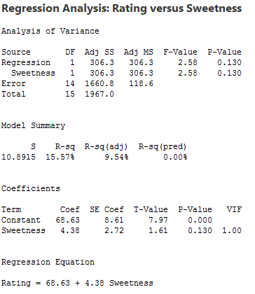
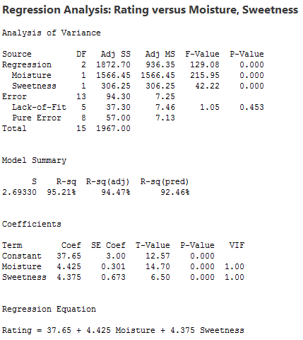
There is a linear relationship between rating and moisture and there is also a sweetness difference. The results given in the following output are for three different regressions - separate simple regressions for each x-variable and a multiple regression that incorporates both x-variables.

There are three important features to notice in the results:

1. The sample coefficient that multiplies Moisture is 4.425 in both the simple and the multiple regression. The sample coefficient that multiplies Sweetness is 4.375 in both the simple and the multiple regression. This result does not generally occur; the only reason that it does in this case is that Moisture and Sweetness are not correlated, so the estimated slopes are independent of each other. For most observational studies, predictors are typically correlated and estimated slopes in a multiple linear regression model do not match the corresponding slope estimates in simple linear regression models.

2. The R² for the multiple regression, 95.21%, is the sum of the R² values for the simple regressions (79.64% and 15.57%). Again, this will only happen when we have uncorrelated x-variables.

3. The variable Sweetness is not statistically significant in the simple regression (p = 0.130), but it is in the multiple regression. This is a benefit of doing a multiple regression. By putting both variables into the equation, we have greatly reduced the standard deviation of the residuals (notice the S values). This in turn reduces the standard errors of the coefficients, leading to greater (absolute) t-values and smaller p-values.

(Data source: Applied Regression Models, (4th edition), Kutner, Neter, and Nachtsheim).

Example 2: Female Stat Students

The data are from n = 214 females in statistics classes at the University of California at Davis (stat_females.txt). The variables are y = student’s self-reported height, x₁ = student’s guess at her mother’s height, and x₂ = student’s guess at her father’s height. All heights are in inches. The scatterplots below are of each student’s height versus mother’s height and student’s height against father’s height.

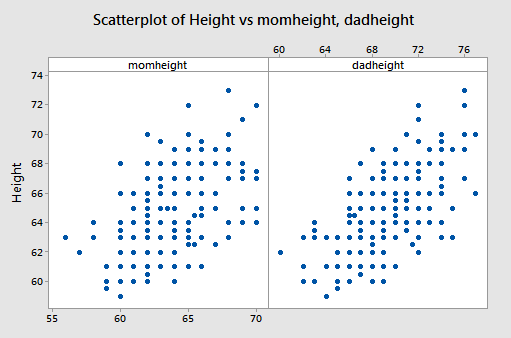
Both show a moderate positive association with a straight-line pattern and no notable outliers.

Interpretations

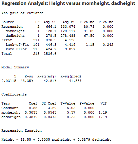
• The sample multiple regression equation is predicted student height = 18.55 + 0.3035 × mother’s height + 0.3879 × father’s height. To use this equation for prediction, we substitute specified values for the two parents’ heights.
• We can interpret the “slopes” in the same way that we do for a simple linear regression model but we have to add the constraint that values of other variables remain constant. For example:
  • When father’s height is held constant, the average student height increases 0.3035 inches for each one-inch increase in mother’s height.
  • When mother’s height is held constant, the average student height increases 0.3879 inches for each one-inch increase in father’s height.
• The p-values given for the two x-variables tell us that student height is significantly related to each.
• The value of R² = 43.35% means that the model (the two x-variables) explains 43.35% of the observed variation in student heights.
• The value S = 2.03115 is the estimated standard deviation of the regression errors. Roughly, it is the average absolute size of a residual.

Residual Plots

Just as in simple regression, we can use a plot of residuals versus fits to evaluate the validity of assumptions. The residual plot for these data is shown in the following figure:

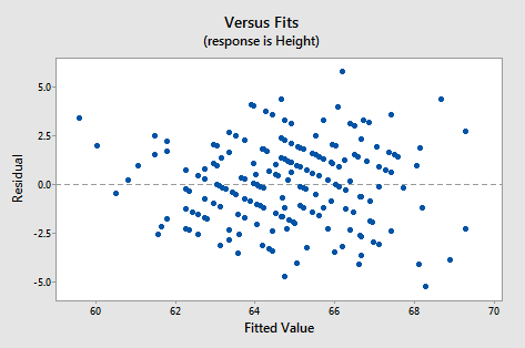
It looks about as it should - a random horizontal band of points. Other residual analyses can be done exactly as we did for simple regression. For instance, we might wish to examine a normal probability plot of the residuals. Additional plots to consider are plots of residuals versus each x-variable separately. This might help us identify sources of curvature or non-constant variance.

Example 3: Hospital Data

Data from n = 113 hospitals in the United States are used to assess factors related to the likelihood that a hospital patients acquires an infection while hospitalized. The variables here are y = infection risk, x₁ = average length of patient stay, x₂ = average patient age, x₃ = measure of how many x-rays are given in the hospital (infectionrisk.txt). Statistical software output is as follows:

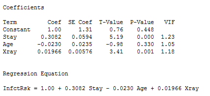
Interpretations for this example include:

• The p-value for testing the coefficient that multiplies Age is 0.330. Thus we cannot reject the null hypothesis H₀: β₂ = 0. The variable Age is not a useful predictor within this model that includes Stay and Xrays.
• For the variables Stay and X-rays, the p-values for testing their coefficients are at a statistically significant level so both are useful predictors of infection risk (within the context of this model!).
• We usually don’t worry about the p-value for Constant. It has to do with the “intercept” of the model and seldom has any practical meaning unless it makes sense for all the x-variables to be zero simultaneously.

(Data source: Applied Regression Models, (4th edition), Kutner, Neter, and Nachtsheim).

Example 4: Physiological Measurements Data

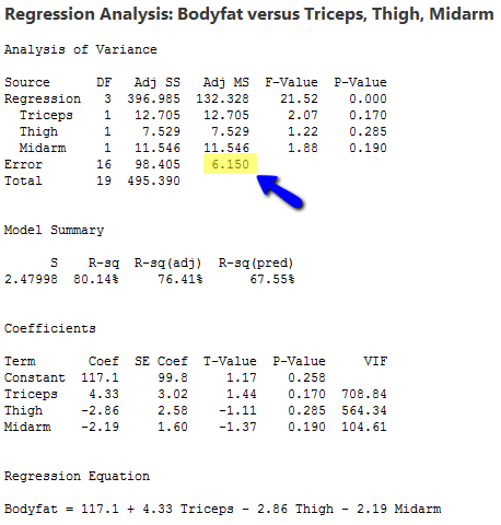
For a sample of n = 20 individuals, we have measurements of y = body fat, x₁ = triceps skinfold thickness, x₂ = thigh circumference, and x₃ = midarm circumference (bodyfat.txt) . Statistical software results for the sample coefficients, MSE (highlighted), and (X^TX)⁻¹ are given below:

(X^TX)⁻¹  - (calculated manually, see note below)

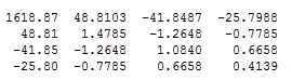
Note: There is no real need to know how to calculate this matrix using statistical software, but in case you're curious first store the design matrix, X from the regression model. Then find the transpose of X and multiply the transpose of X and X. Finally, invert the resulting matrix.

The variance-covariance matrix of the sample coefficients is found by multiplying each element in  (X^TX)⁻¹ by MSE. Common notation for the resulting matrix is either s²(b) or se²(b). Thus, the standard errors of the coefficients given in the output above can be calculated as follows:

• Var(b₀) = (6.15031)(1618.87) = 9956.55, so se(b₀) = \(\sqrt{9956.55}\) = 99.782.
• Var(b₁) = (6.15031)(1.4785) = 9.0932, so se(b₁) = \(\sqrt{9.0932}\) = 3.016.
• Var(b₂) = (6.15031)(1.0840) = 6.6669, so se(b₂) = \(\sqrt{6.6669}\) = 2.582.
• Var(b₃) = (6.15031)(0.4139) = 2.54561, so se(b₃) = \(\sqrt{2.54561}\) = 1.595.

As an example of a covariance and correlation between two coefficients, we consider b₁ and b₂.

• Cov(b₁, b₂) = (6.15031)(−1.2648) = −7.7789. The value -1.2648 is in the second row and third column of  (X^TX)⁻¹. (Keep in mind that the first row and first column give information about b₀, so the second row has information about b₁, and so on.)
• Corr(b₁, b₂) = covariance divided by product of standard errors = −7.7789 / (3.016 × 2.582) = −0.999.

The extremely high correlation between these two sample coefficient estimates results from a high correlation between the Triceps and Thigh variables. The consequence is that it is difficult to separate the individual effects of these two variables.

If all x-variables are uncorrelated with each other, then all covariances between pairs of sample coefficients that multiply x-variables will equal 0. This means that the estimate of one beta is not affected by the presence of the other x-variables. Many experiments are designed to achieve this property. With observational data, however, we’ll most likely not have this happen.

(Data source: Applied Regression Models, (4th edition), Kutner, Neter, and Nachtsheim).

Example 5: Peruvian Blood Pressure Data

This dataset consists of variables possibly relating to blood pressures of n = 39 Peruvians who have moved from rural high altitude areas to urban lower altitude areas (peru.txt). The variables in this dataset are:

Y = systolic blood pressure
X₁ = age
X₂ = years in urban area
X₃ = X₂ /X₁ = fraction of life in urban area
X₄ = weight (kg)
X₅ = height (mm)
X₆ = chin skinfold
X₇ = forearm skinfold
X₈ = calf skinfold
X₉  = resting pulse rate

First, we run a multiple regression using all nine x-variables as predictors. The results are given below.

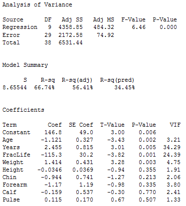
When looking at tests for individual variables, we see that p-values for the variables Height, Chin, Forearm, Calf, and Pulse are not at a statistically significant level. These individual tests are affected by correlations amongst the x-variables, so we will use the general linear F-test to see whether it is reasonable to declare that all five non-significant variables can be dropped from the model.

In other words, consider testing:

H₀ : β₅ = β₆ = β₇ = β₈ = β₉ = 0
H_A : at least one of {β₅ , β₆ , β₇ , β₈ , β₉ } ≠ 0

within the nine variable model given above. If this null is not rejected, it is reasonable to say that none of the five variables Height, Chin, Forearm, Calf and Pulse contribute to the prediction/explanation of systolic blood pressure.

The full model includes all nine variables; SSE(full) = 2172.58, the full error df = 29, and MSE(full) = 74.92 (we get these from the results above). The reduced model includes only the variables Age, Years, fraclife, and Weight (which are the remaining variables if the five possibly non-significant variables are dropped). Regression results for the reduced model are given below.

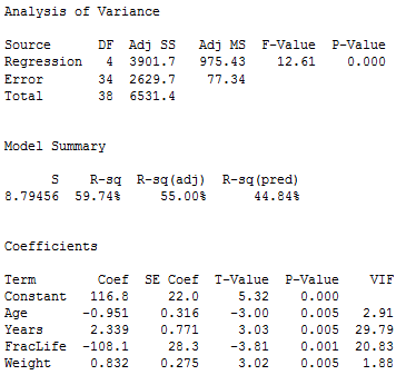
We see that SSE(reduced) = 2629.7, and the reduced error df = 34. We also see that all four individual x-variables are statistically significant.

The calculation for the general linear F-test statistic is:

\[F=\frac{\frac{\text{SSE(reduced) - SSE(full)}}{\text{error df for reduced - error df for full}}}{\text{MSE(full)}}=\frac{\frac{2629.7-2172.58}{34-29}}{74.92}=1.220\]

Thus, this test statistic comes from an F_5,29 distribution, of which the associated p-value is 0.325 (this can be found by using statistical software or looking up a table). This is not at a statistically significant level, so we do not reject the null hypothesis and we favour the reduced model. Thus it is feasible to drop the variables X₅, X₆, X₇, X₈, and X₉ from the model.

Example 6: Measurements of College Students

For n = 55 college students, we have measurements (Physical.txt) for the following five variables:

Y = height (in)
X₁ = left forearm length (cm)
X₂ = left foot length (cm)
X₃ = head circumference (cm)
X₄ = nose length (cm)

Statistical software output for the full model is given below.

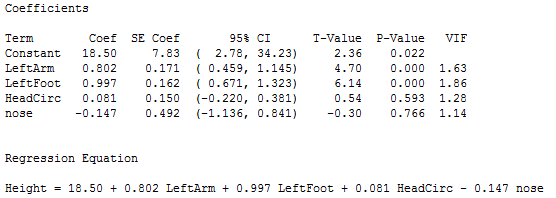
The interpretations of the t-tests are as follows:

• The sample coefficients for LeftArm and LeftFoot achieve statistical significance. This indicates that they are useful as predictors of Height.
• The sample coefficients for HeadCirc and nose are not significant. Each t-test considers the question of whether the variable is needed, given that all other variables will remain in the model.

Below is a plot of residuals versus the fitted values and it seems suitable.

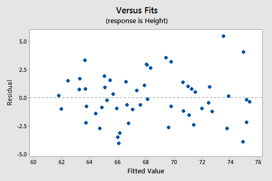
There is no obvious curvature and the variance is reasonably constant. One may note two possible outliers, but nothing serious.

The first calculation we will perform is for the general linear F-test. The results above might lead us to test

H₀ : β₃ = β₄ = 0
H_A : at least one of {β₃ , β₄} ≠ 0

in the full model. If we fail to reject the null hypothesis, we could then remove both of HeadCirc and nose as predictors.

Below is the ANOVA table for the full model.

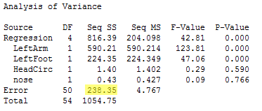
From this output, we see that SSE(full) = 238.35, with df = 50, and MSE(full) = 4.77. The reduced model includes only the two variables LeftArm and LeftFoot as predictors. The ANOVA results for the reduced model are found below.

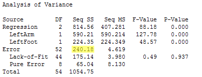
From this output, we see that SSE(reduced) = SSE(X₁ , X₂) = 240.18, with df = 52, and MSE(reduced) = MSE(X₁ , X₂) = 4.62.

With these values obtained, we can now obtain the test statistic for testing H₀ : β₃ = β₄ = 0:

\[F=\frac{\frac{\text{SSE(X_1, X_2) - SSE(full)}}{\text{error df for reduced - error df for full}}}{\text{MSE(full)}}=\frac{\frac{240.18-238.35}{52-50}}{4.77}=0.192\]

This value comes from an F_2,50 distribution. By using statistical software or looking up a table we find that the area to the left of F = 0.192 (with df of 2 and 50) is 0.174. The p-value is the area to the right of F, so p = 1 − 0.174 = 0.826. Thus, we do not reject the null hypothesis, we favour the reduced model, and it is reasonable to remove HeadCirc and nose from the model.

Next we consider what fraction of variation in Y = Height cannot be explained by X₂ = LeftFoot, but can be explained by X₁ = LeftArm? To answer this question, we calculate the partial R². The formula is:

\[R_{Y, 1|2}^{2}=\frac{SSR(X_1|X_2)}{SSE(X_2)}=\frac{SSE(X_2)-SSE(X_1,X_2)}{SSE(X_2)}\]

The denominator, SSE(X₂), measures the unexplained variation in Y when X₂ is the predictor. The ANOVA table for this regression is found in below.

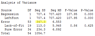
These results give us SSE(X₂) = 347.3.

The numerator, SSE(X₂)–SSE(X₁,  X₂ ), measures the further reduction in the SSE when X₁ is added to the model. Results from the earlier output give us SSE(X₁,  X₂ ) = 240.18 and now we can calculate:

\[R_{Y, 1|2}^{2}=\frac{SSR(X_1|X_2)}{SSE(X_2)}=\frac{SSE(X_2)-SSE(X_1,X_2)}{SSE(X_2)}=\frac{347.3-240.18}{347.3}=0.308\]

Thus X₁ = LeftArm explains 30.8% of the variation in Y = Height that could not be explained by X₂ = LeftFoot.