Note: This portion of the lesson is most important for those students who will continue studying statistics after taking Stat 462. We will only rarely use the material within the remainder of this course.

A matrix formulation of the multiple regression model

In the multiple regression setting, because of the potentially large number of predictors, it is more efficient to use matrices to define the regression model and the subsequent analyses. Here, we review basic matrix algebra, as well as learn some of the more important multiple regression formulas in matrix form.

As always, let's start with the simple case first. Consider the following simple linear regression function:

\[y_i=\beta_0+\beta_1x_i+\epsilon_i  \;\;\;\;\;\;\; \text {for } i=1, ... , n\]

If we actually let i = 1, ..., n, we see that we obtain n equations:

\[\begin{align}
y_1 & =\beta_0+\beta_1x_1+\epsilon_1 \\
y_2 & =\beta_0+\beta_1x_2+\epsilon_2 \\
\vdots \\
y_n & = \beta_0+\beta_1x_n+\epsilon_n
\end{align}\]

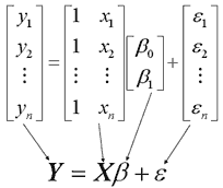
Well, that's a pretty inefficient way of writing it all out! As you can see, there is a pattern that emerges. By taking advantage of this pattern, we can instead formulate the above simple linear regression function in matrix notation:

That is, instead of writing out the n equations, using matrix notation, our simple linear regression function reduces to a short and simple statement:

\[Y=X\beta+\epsilon\]

Now, what does this statement mean? Well, here's the answer:

• X is an n × 2 matrix.
• Y is an n × 1 column vector, β is a 2 × 1 column vector, and ε is an n × 1 column vector.
• The matrix X and vector β are multiplied together using the techniques of matrix multiplication.
• And, the vector Xβ is added to the vector ε using the techniques of matrix addition.

Now, that might not mean anything to you, if you've never studied matrix algebra — or if you have and you forgot it all! So, let's start with a quick and basic review.

Definition of a matrix

An r × c matrix is a rectangular array of symbols or numbers arranged in r rows and c columns. A matrix is almost always denoted by a single capital letter in boldface type.

Here are three examples of simple matrices. The matrix A is a 2 × 2 square matrix containing numbers:

\[A=\begin{bmatrix}
 1&2 \\
6 & 3
\end{bmatrix}\]

The matrix B is a 5 × 3 matrix containing numbers:

\[B=\begin{bmatrix}
1 & 80 &3.4\\
1 & 92 & 3.1\\
1 & 65 &2.5\\
1 &71  & 2.8\\
1 & 40 & 1.9
\end{bmatrix}\]

And, the matrix X is a 6 × 3 matrix containing a column of 1's and two columns of various x variables:

\[X=\begin{bmatrix}
1 & x_{11}&x_{12}\\
1 & x_{21}& x_{22}\\
1 & x_{31}&x_{32}\\
1 &x_{41}& x_{42}\\
1 & x_{51}& x_{52}\\
1 & x_{61}& x_{62}\\
\end{bmatrix}\]

Definition of a vector and a scalar

A column vector is an r × 1 matrix, that is, a matrix with only one column. A vector is almost often denoted by a single lowercase letter in boldface type. The following vector q is a 3 × 1 column vector containing numbers:

\[q=\begin{bmatrix}
2\\
5\\
8\end{bmatrix}\]

A row vector is an 1 × c matrix, that is, a matrix with only one row. The vector h is a 1 × 4 row vector containing numbers:

\[h=\begin{bmatrix}
21 &46  & 32 & 90
\end{bmatrix}\]

A 1 × 1 "matrix" is called a scalar, but it's just an ordinary number, such as 29 or σ².

Matrix multiplication

Recall that Xβ that appears in the regression function:

\[Y=X\beta+\epsilon\]

is an example of matrix multiplication. Now, there are some restrictions — you can't just multiply any two old matrices together. Two matrices can be multiplied together only if the number of columns of the first matrix equals the number of rows of the second matrix. Then, when you multiply the two matrices:

• the number of rows of the resulting matrix equals the number of rows of the first matrix, and
• the number of columns of the resulting matrix equals the number of columns of the second matrix.

For example, if A is a 2 × 3 matrix and B is a 3 × 5 matrix, then the matrix multiplication AB is possible. The resulting matrix C = AB has 2 rows and 5 columns. That is, C is a 2 × 5 matrix. Note that the matrix multiplication BA is not possible.

For another example, if X is an n × (k+1) matrix and β is a (k+1) × 1 column vector, then the matrix multiplication Xβ is possible. The resulting matrix Xβ has n rows and 1 column. That is, Xβ is an n × 1 column vector.

Okay, now that we know when we can multiply two matrices together, how do we do it? Here's the basic rule for multiplying A by B to get C = AB:

The entry in the i^th row and j^th column of C is the inner product — that is, element-by-element products added together — of the i^th row of A with the j^th column of B.

For example:

\[C=AB=\begin{bmatrix}
1&9&7 \\
8&1&2
\end{bmatrix}\begin{bmatrix}
3&2&1&5 \\
5&4&7&3 \\
6&9&6&8
\end{bmatrix}=\begin{bmatrix}
90&101&106&88 \\
41&38&27&59
\end{bmatrix}\]

That is, the entry in the first row and first column of C, denoted c₁₁, is obtained by:

\[c_{11}=1(3)+9(5)+7(6)=90\]

And, the entry in the first row and second column of C, denoted c₁₂, is obtained by:

\[c_{12}=1(2)+9(4)+7(9)=101\]

And, the entry in the second row and third column of C, denoted c₂₃, is obtained by:

\[c_{23}=8(1)+1(7)+2(6)=27\]

You might convince yourself that the remaining five elements of C have been obtained correctly.

Matrix addition

Recall that Xβ + ε that appears in the regression function:

\[Y=X\beta+\epsilon\]

is an example of matrix addition. Again, there are some restrictions — you can't just add any two old matrices together. Two matrices can be added together only if they have the same number of rows and columns. Then, to add two matrices, simply add the corresponding elements of the two matrices. That is:

• Add the entry in the first row, first column of the first matrix with the entry in the first row, first column of the second matrix.
• Add the entry in the first row, second column of the first matrix with the entry in the first row, second column of the second matrix.
• And, so on.

For example:

\[C=A+B=\begin{bmatrix}
 2&4&-1\\
 1&8&7\\
3&5&6
\end{bmatrix}+\begin{bmatrix}
7 & 5 & 2\\
9 & -3 & 1\\
2 & 1 & 8
\end{bmatrix}=\begin{bmatrix}
9 & 9 & 1\\
10 & 5 & 8\\
5 & 6 & 14
\end{bmatrix}\]

That is, the entry in the first row and first column of C, denoted c₁₁, is obtained by:

\[c_{11}=2+7=9\]

And, the entry in the first row and second column of C, denoted c₁₂, is obtained by:

\[c_{12}=4+5=9\]

You might convince yourself that the remaining seven elements of C have been obtained correctly.

Least squares estimates in matrix notation

Here's the punchline: the (k+1) × 1 vector containing the estimates of the (k+1) parameters of the regression function can be shown to equal:

\[ b=\begin{bmatrix}
b_0 \\
b_1 \\
\vdots \\
b_{k} \end{bmatrix}= (X^{'}X)^{-1}X^{'}Y \]

where:

• (X'X)^–1 is the inverse of the X'X matrix, and
• X' is the transpose of the X matrix.

As before, that might not mean anything to you, if you've never studied matrix algebra — or if you have and you forgot it all! So, let's go off and review inverses and transposes of matrices.

Definition of the transpose of a matrix

The transpose of a matrix A is a matrix, denoted A' or A^T, whose rows are the columns of A and whose columns are the rows of A — all in the same order. For example, the transpose of the 3 × 2 matrix A:

\[A=\begin{bmatrix}
 1&5 \\
 4&8 \\
 7&9
\end{bmatrix}\]

is the 2 × 3 matrix A':

\[A^{'}=A^T=\begin{bmatrix}
 1& 4 & 7\\
5 & 8 & 9 \end{bmatrix}\]

And, since the X matrix in the simple linear regression setting is:

\[X=\begin{bmatrix}
1 & x_1\\
1 & x_2\\
\vdots & \vdots\\
1 & x_n
\end{bmatrix}\]

the X'X matrix in the simple linear regression setting must be:

\[X^{'}X=\begin{bmatrix}
1 & 1 & \cdots & 1\\
x_1 & x_2 & \cdots & x_n
\end{bmatrix}\begin{bmatrix}
1 & x_1\\
1 & x_2\\
\vdots &  x_n\\ 
1&  
\end{bmatrix}=\begin{bmatrix}
n & \sum_{i=1}^{n}x_i \\
\sum_{i=1}^{n}x_i  & \sum_{i=1}^{n}x_{i}^{2}
\end{bmatrix}\]

Definition of the identity matrix

The square n × n identity matrix, denoted I_n, is a matrix with 1's on the diagonal and 0's elsewhere. For example, the 2 × 2 identity matrix is:

\[I_2=\begin{bmatrix}
1 & 0\\
0 & 1
\end{bmatrix}\]

The identity matrix plays the same role as the number 1 in ordinary arithmetic:

\[\begin{bmatrix}
9 & 7\\
4& 6
\end{bmatrix}\begin{bmatrix}
1 & 0\\
0 & 1
\end{bmatrix}=\begin{bmatrix}
9& 7\\
4& 6
\end{bmatrix}\]

That is, when you multiply a matrix by the identity, you get the same matrix back.

Definition of the inverse of a matrix

The inverse A^-1 of a square (!!) matrix A is the unique matrix such that:

\[A^{-1}A = I = AA^{-1}\]

That is, the inverse of A is the matrix A^-1 that you have to multiply A by in order to obtain the identity matrix I. Note that I am not just trying to be cute by including (!!) in that first sentence. The inverse only exists for square matrices!

Now, finding inverses is a really messy venture. The good news is that we'll always let computers find the inverses for us. In fact, we won't even know that statistical software is finding inverses behind the scenes!

An example

Ugh! All of these definitions! Let's take a look at an example just to convince ourselves that, yes, indeed the least squares estimates are obtained by the following matrix formula:

\[b=\begin{bmatrix}
b_0\\
b_1\\
\vdots\\
b_{p-1}
\end{bmatrix}=(X^{'}X)^{-1}X^{'}Y\]

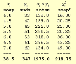
Let's consider the data in soapsuds.txt, in which the height of suds (y = suds) in a standard dishpan was recorded for various amounts of soap (x = soap, in grams) (Draper and Smith, 1998, p. 108). Using statistical software to fit the simple linear regression model to these data, we obtain:

Let's see if we can obtain the same answer using the above matrix formula. We previously showed that:

\[X^{'}X=\begin{bmatrix}
n & \sum_{i=1}^{n}x_i \\
\sum_{i=1}^{n}x_i  & \sum_{i=1}^{n}x_{i}^{2}
\end{bmatrix}\]

We can easily calculate some parts of this formula:

That is, the 2 × 2 matrix X'X is:

\[X^{'}X=\begin{bmatrix}
7 & 38.5\\
38.5& 218.75
\end{bmatrix}\]

And, the 2 × 1 column vector X'Y is:

\[X^{'}Y=\begin{bmatrix}
\sum_{i=1}^{n}y_i\\
\sum_{i=1}^{n}x_iy_i
\end{bmatrix}=\begin{bmatrix}
347\\
1975
\end{bmatrix}\]

So, we've determined X'X and X'Y. Now, all we need to do is to find the inverse (X'X)^-1. As mentioned before, it is very messy to determine inverses by hand. Letting computer software do the dirty work for us, it can be shown that the inverse of X'X is:

\[(X^{'}X)^{-1}=\begin{bmatrix}
4.4643 & -0.78571\\
-0.78571& 0.14286
\end{bmatrix}\]

And so, putting all of our work together, we obtain the least squares estimates:

\[b=(X^{'}X)^{-1}X^{'}Y=\begin{bmatrix}
4.4643 & -0.78571\\
-0.78571& 0.14286
\end{bmatrix}\begin{bmatrix}
347\\
1975
\end{bmatrix}=\begin{bmatrix}
-2.67\\
9.51
\end{bmatrix}\]

That is, the estimated intercept is b₀ = -2.67 and the estimated slope is b₁ = 9.51. Aha! Our estimates are the same as those reported above (within rounding error)!

Further Matrix Results for Multiple Linear Regression

Matrix notation applies to other regression topics, including fitted values, residuals, sums of squares, and inferences about regression parameters. One important matrix that appears in many formulas is the so-called "hat matrix," \(H = X(X^{'}X)^{-1}X^{'}\), since it puts the hat on \(Y\)!

Linear Dependence

There is just one more really critical topic that we should address here, and that is linear dependence. We say that the columns of the matrix A:

\[A=\begin{bmatrix}
 1& 2 & 4 &1 \\
2 & 1 & 8 & 6\\
3 & 6 & 12 & 3
\end{bmatrix}\]

are linearly dependent, since (at least) one of the columns can be written as a linear combination of another, namely the third column is 4 × the first column. If none of the columns can be written as a linear combination of the other columns, then we say the columns are linearly independent.

Unfortunately, linear dependence is not always obvious. For example, the columns in the following matrix A:

\[A=\begin{bmatrix}
 1& 4 & 1 \\
2 & 3 & 1\\
3 & 2 & 1
\end{bmatrix}\]

are linearly dependent, because the first column plus the second column equals 5 × the third column.

Now, why should we care about linear dependence? Because the inverse of a square matrix exists only if the columns are linearly independent. Since the vector of regression estimates b depends on (X'X)^-1, the parameter estimates b₀, b₁, and so on cannot be uniquely determined if some of the columns of X are linearly dependent! That is, if the columns of your X matrix — that is, two or more of your predictor variables — are linearly dependent (or nearly so), you will run into trouble when trying to estimate the regression equation.

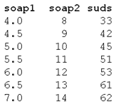
For example, suppose for some strange reason we multiplied the predictor variable soap by 2 in the dataset soapsuds.txt. That is, we'd have two predictor variables, say soap1 (which is the original soap) and soap2 (which is 2 × the original soap):

If we tried to regress y = suds on x₁ = soap1 and x₂ = soap2, we see that statistical software spits out trouble:

In short, the first moral of the story is "don't collect your data in such a way that the predictor variables are perfectly correlated." And, the second moral of the story is "if your software package reports an error message concerning high correlation among your predictor variables, then think about linear dependence and how to get rid of it."