Earlier in this lesson, we translated three different research questions pertaining to the heart attacks in rabbits study (coolhearts.txt) into three sets of hypotheses we can test using the general linear F-statistic. The research questions and their corresponding hypotheses are:

1. Is the regression model containing at least one predictor useful in predicting the size of the infarct?

• H₀ : β₁ = β₂ = β₃ = 0
• H_A : At least one β_j ≠ 0 (for j = 1, 2, 3)

2. Is the size of the infarct significantly (linearly) related to the area of the region at risk?

• H₀ : β₁ = 0
• H_A : β₁ ≠ 0

3. (Primary research question) Is the size of the infarct area significantly (linearly) related to the type of treatment upon controlling for the size of the region at risk for infarction?

• H₀ : β₂ = β₃ = 0
• H_A : At least one β_j ≠ 0 (for j = 2, 3)

Let's test each of the hypotheses now using the general linear F-statistic:

\[F^*=\left(\frac{SSE(R)-SSE(F)}{df_R-df_F}\right) \div \left(\frac{SSE(F)}{df_F}\right)\]

To calculate the F-statistic for each test, we first determine the error sum of squares for the reduced and full models — SSE(R) and SSE(F), respectively. The number of error degrees of freedom associated with the reduced and full models — df_R and df_F, respectively — is the number of observations, n, minus the number of parameters, k+1, in the model. That is, in general, the number of error degrees of freedom is n – (k+1). We use statistical software to determine the P-value for each test.

Testing all slope parameters equal 0

To answer the research question: "Is the regression model containing at least one predictor useful in predicting the size of the infarct?," we test the hypotheses:

• H₀ : β₁ = β₂ = β₃ = 0
• H_A : At least one β_j ≠ 0 (for j = 1, 2, 3)

The full model. The full model is the largest possible model — that is, the model containing all of the possible predictors. In this case, the full model is:

\[y_i=(\beta_0+\beta_1x_{i1}+\beta_2x_{i2}+\beta_3x_{i3})+\epsilon_i\]

The error sum of squares for the full model, SSE(F), is just the usual error sum of squares, SSE, that appears in the analysis of variance table. Because there are k+1 = 3+1 = 4 parameters in the full model, the number of error degrees of freedom associated with the full model is df_F = n – 4.

The reduced model. The reduced model is the model that the null hypothesis describes. Because the null hypothesis sets each of the slope parameters in the full model equal to 0, the reduced model is:

\[y_i=\beta_0+\epsilon_i\]

The reduced model basically suggests that none of the variation in the response y is explained by any of the predictors. Therefore, the error sum of squares for the reduced model, SSE(R), is just the total sum of squares, SSTO, that appears in the analysis of variance table. Because there is only one parameter in the reduced model, the number of error degrees of freedom associated with the reduced model is df_R = n – 1.

The test. Upon plugging in the above quantities, the general linear F-statistic:

\[F^*=\frac{SSE(R)-SSE(F)}{df_R-df_F} \div \frac{SSE(F)}{df_F}\]

becomes the usual "overall F-test":

\[F^*=\frac{SSR}{3} \div \frac{SSE}{n-4}=\frac{MSR}{MSE}.\]

That is, to test H₀ : β₁ = β₂ = β₃ = 0, we just use the overall F-test and P-value reported in the analysis of variance table:

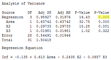
\[F^*=\frac{0.95927}{3} \div \frac{0.54491}{28}=\frac{0.31976}{0.01946}=16.43.\]

There is sufficient evidence (F = 16.43, P < 0.001) to conclude that at least one of the slope parameters is not equal to 0.

In general, to test that all of the slope parameters in a multiple linear regression model are 0, we use the overall F-test reported in the analysis of variance table.

Testing one slope parameter is 0

Now let's answer the second research question: "Is the size of the infarct significantly (linearly) related to the area of the region at risk?" To do so, we test the hypotheses:

• H₀ : β₁ = 0
• H_A : β₁ ≠ 0

The full model. Again, the full model is the model containing all of the possible predictors:

\[y_i=(\beta_0+\beta_1x_{i1}+\beta_2x_{i2}+\beta_3x_{i3})+\epsilon_i\]

The error sum of squares for the full model, SSE(F), is just the usual error sum of squares, SSE. Alternatively, because the three predictors in the model are x₁, x₂, and x₃, we can denote the error sum of squares as SSE(x₁, x₂, x₃). Again, because there are 4 parameters in the model, the number of error degrees of freedom associated with the full model is df_F = n – 4.

The reduced model. Because the null hypothesis sets the first slope parameter, β₁, equal to 0, the reduced model is:

\[y_i=(\beta_0+\beta_2x_{i2}+\beta_3x_{i3})+\epsilon_i\]

Because the two predictors in the model are x₂ and x₃, we denote the error sum of squares as SSE(x₂, x₃). Because there are 3 parameters in the model, the number of error degrees of freedom associated with the reduced model is df_R = n – 3.

The test. The general linear statistic:

\[F^*=\frac{SSE(R)-SSE(F)}{df_R-df_F} \div \frac{SSE(F)}{df_F}\]

simplifies to:

\[F^*=\frac{SSR(x_1|x_2, x_3)}{1}\div \frac{SSE(x_1,x_2, x_3)}{n-4}=\frac{MSR(x_1|x_2, x_3)}{MSE(x_1,x_2, x_3)}\]

Getting the numbers from the following output:

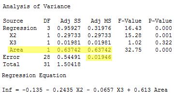
we determine that value of the F-statistic is:

\[F^*=\frac{SSR(x_1|x_2, x_3)}{1}\div MSE=\frac{0.63742}{0.01946}=32.7554.\]

The P-value is the probability — if the null hypothesis were true — that we would get an F-statistic larger than 32.7554. Comparing our F-statistic to an F-distribution with 1 numerator degree of freedom and 28 denominator degrees of freedom, the probability is close to 1 that we would observe an F-statistic smaller than 32.7554:

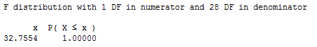
Therefore, the probability that we would get an F-statistic larger than 32.7554 is close to 0. That is, the P-value is < 0.001. There is sufficient evidence (F = 32.8, P < 0.001) to conclude that the size of the infarct is significantly related to the size of the area at risk.

But wait a second! Have you been wondering why we couldn't just use the slope's t-statistic to test that the slope parameter, β₁, is 0? We can! Notice that the P-value (P < 0.001) for the t-test (t* = 5.72):

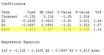
is the same as the P-value we obtained for the F-test. This will be always be the case when we test that only one slope parameter is 0. That's because of the well-known relationship between a t-statistic and an F-statistic that has one numerator degree of freedom:

\[t_{(n-(k+1))}^{2}=F_{(1, n-(k+1))}\]

For our example, the square of the t-statistic, 5.72, equals our F-statistic (within rounding error). That is:

\[t^{*2}=5.72^2=32.72=F^*\]

So what have we learned in all of this discussion about the equivalence of the F-test when testing only one slope parameter and the t-test? In short:

• We can use either the F-test or the t-test to test that only one slope parameter is 0. Because the t-test results can be read directly from the software output, it makes sense that it would be the test that we'll use most often.
• But, we have to be careful with our interpretations! The equivalence of the t-test to the F-test when testing only one slope parameter has taught us something new about the t-test. The t-test is a test for the marginal significance of the x₁ predictor after the other predictors x₂ and x₃ have been taken into account. It does not test for the significance of the relationship between the response y and the predictor x₁ alone.

Testing a subset of slope parameters is 0

Finally, let's answer the third — and primary — research question: "Is the size of the infarct area significantly (linearly) related to the type of treatment upon controlling for the size of the region at risk for infarction?" To do so, we test the hypotheses:

• H₀ : β₂ = β₃ = 0
• H_A : At least one β_j ≠ 0 (for j = 2, 3)

The full model. Again, the full model is the model containing all of the possible predictors:

\[y_i=(\beta_0+\beta_1x_{i1}+\beta_2x_{i2}+\beta_3x_{i3})+\epsilon_i\]

The error sum of squares for the full model, SSE(F), is just the usual error sum of squares, SSE = 0.54491 from the output above. Alternatively, because the three predictors in the model are x₁, x₂, and x₃, we can denote the error sum of squares as SSE(x₁, x₂, x₃). Again, because there are 4 parameters in the model, the number of error degrees of freedom associated with the full model is df_F = n – 4 = 32 – 4 = 28.

The reduced model. Because the null hypothesis sets the second and third slope parameters, β₂ and β₃, equal to 0, the reduced model is:

\[y_i=(\beta_0+\beta_1x_{i1})+\epsilon_i\]

The ANOVA table for the reduced model is:

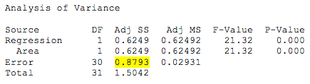
Because the only predictor in the model is x₁, we denote the error sum of squares as SSE(x₁) = 0.8793. Because there are 2 parameters in the model, the number of error degrees of freedom associated with the reduced model is df_R = n – 2 = 32 – 2 = 30.

The test. The general linear statistic is:

\[F^*=\frac{SSE(R)-SSE(F)}{df_R-df_F} \div\frac{SSE(F)}{df_F}=\frac{0.8793-0.54491}{30-28} \div\frac{0.54491}{28}= \frac{0.33439}{2} \div 0.01946=8.59.\]

The P-value is the probability — if the null hypothesis were true — that we would observe an F-statistic more extreme than 8.59. The following output:

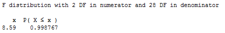
tells us that the probability of observing such an F-statistic that is smaller than 8.59 is 0.9988. Therefore, the probability of observing such an F-statistic that is larger than 8.59 is 1 – 0.9988 = 0.0012. The P-value is very small. There is sufficient evidence (F = 8.59, P = 0.0012) to conclude that the type of cooling is significantly related to the extent of damage that occurs — after taking into account the size of the region at risk.

Summary of MLR Testing

For the simple linear regression model, there is only one slope parameter about which one can perform hypothesis tests. For the multiple linear regression model, there are three different hypothesis tests for slopes that one could conduct. They are:

• Hypothesis test for testing that all of the slope parameters are 0.
• Hypothesis test for testing that a subset — more than one, but not all — of the slope parameters are 0.
• Hypothesis test for testing that one slope parameter is 0.

We have learned how to perform each of the above three hypothesis tests.

The F-statistic and associated p-value in the ANOVA table are used for testing whether all of the slope parameters are 0. In most applications this p-value will be small enough to reject the null hypothesis and conclude that at least one predictor is useful in the model. For example, for the rabbit heart attacks study, the F-statistic is (0.95927/3) / (0.54491/(32–4)) = 16.43 with p-value 0.000.

To test whether a subset — more than one, but not all — of the slope parameters are 0, use the general linear F-test formula by fitting the full model to find SSE(F) and fitting the reduced model to find SSE(R). Then the numerator of the F-statistic is (SSE(R) – SSE(F)) / (df_R – df_F). The denominator of the F-statistic is the mean squared error in the ANOVA table. For example, for the rabbit heart attacks study, the general linear F-statistic is [(0.8793 – 0.54491) / (30 – 28)] / (0.54491 / 28) = 8.59 with p-value 0.0012.

To test whether one slope parameter is 0, we can use an F-test as just described. Alternatively, we can use a t-test, which will have an identical p-value since in this case the square of the t-statistic is equal to the F-statistic. For example, for the rabbit heart attacks study, the F-statistic for testing the slope parameter for the Area predictor is (0.63742/1) / (0.54491/(32–4)) = 32.75 with p-value 0.000. Alternatively, the t-statistic for testing the slope parameter for the Area predictor is 0.613 / 0.107 = 5.72 with p-value 0.000, and 5.72² = 32.72.

Incidentally, you may be wondering why we can't just do a series of individual t-tests to test whether a subset of the slope parameters are 0. For example, for the rabbit heart attacks study, we could have done the following:

• Fit the model of y = InfSize on x₁ = Area and x₂ and x₃ and use an individual t-test for x₃.
• If the test results indicate that we can drop x₃ then fit the model of y = InfSize on x₁ = Area and x₂ and use an individual t-test for x₂.

The problem with this approach is we're using two individual t-tests instead of one F-test, which means our chance of drawing an incorrect conclusion in our testing procedure is higher. Every time we do a hypothesis test, we can draw an incorrect conclucion by:

• rejecting a true null hypothesis, i.e., make a type 1 error by concluding the tested predictor(s) should be retained in the model, when in truth it/they should be dropped; or
• failing to reject a false null hypothesis, i.e., make a type 2 error by concluding the tested predictor(s) should be dropped from the model, when in truth it/they should be retained.

Thus, in general, the fewer tests we perform the better. In this case, this means that wherever possible using one F-test in place of multiple individual t-tests is preferable.