7.1 - Log-transforming Only the Predictor for SLR
In this section, we learn how to build and use a simple linear regression model by transforming the predictor x values. This might be the first thing that you try if you find a non-linear trend in your data. That is, transforming the x values is appropriate when non-linearity is the only problem (i.e., the independence, normality, and equal variance conditions are met). Note, though, that it may be necessary to correct the non-linearity before you can assess the normality and equal variance assumptions. Also, while some assumptions may appear to hold prior to applying a transformation, they may no longer hold once a transformation is applied. In other words, using transformations is part of an iterative process where all the linear regression assumptions are re-checked after each iteration.
Keep in mind that although we're focussing on a simple linear regression model here, the essential ideas apply more generally to multiple linear regression models too. We can consider transforming any of the predictors by examining scatterplots of the residuals versus each predictor in turn.
Building the model
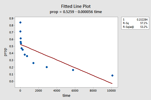
An example. The easiest way to learn about data transformations is by example. Let's consider the data from a memory retention experiment in which 13 subjects were asked to memorize a list of disconnected items. The subjects were then asked to recall the items at various times up to a week later. The proportion of items (y = prop) correctly recalled at various times (x = time, in minutes) since the list was memorized were recorded (wordrecall.txt) and plotted. Recognizing that there is no good reason that the error terms would not be independent, let's evaluate the remaining three conditions — linearity, normality, and equal variances — of the model.
The resulting fitted line plot suggests that the proportion of recalled items (y) is not linearly related to time (x):
The residuals vs. fits plot also suggests that the relationship is not linear:
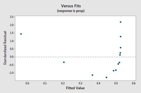
Because the lack of linearity dominates the plot, we cannot use the plot to evaluate whether or not the error variances are equal. We have to fix the non-linearity problem before we can assess the assumption of equal variances.
What about the normal probability plot of the residuals? What does it suggest about the error terms? Can we conclude that they are normally distributed?
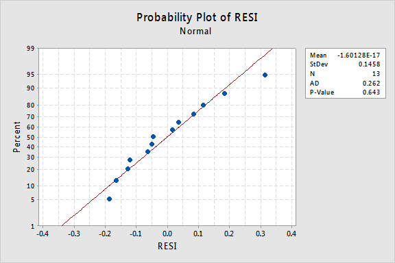
The Anderson-Darling P-value for this example is 0.643, which suggests that we fail to reject the null hypothesis of normal error terms. There is not enough evidence to conclude that the errors terms are not normal.
In summary, we have a data set in which non-linearity is the only major problem. This situation screams out for transforming only the predictor's values. Before we do so, let's take an aside and discuss the "logarithmic transformation," since it is the most common and most useful data transformation available.
The logarithmic transformation. The default logarithmic transformation merely involves taking the natural logarithm — denoted ln or loge or simply log — of each data value. One could consider taking a different kind of logarithm, such as log base 10 or log base 2. However, the natural logarithm — which can be thought of as log base e where e is the constant 2.718282... — is the most common logarithmic scale used in scientific work.
The general characteristics of the natural logarithmic function are:
- The natural logarithm of x is the power of e = 2.718282... that you have to take in order to get x. This can be stated notationally as ln(ex) = x. For example, the natural logarithm of 5 is the power to which you have to raise e = 2.718282... in order to get 5. Since 2.7182821.60944 is approximately 5, we say that the natural logarithm of 5 is 1.60944. Notationally, we say ln(5) = 1.60944.
- The natural logarithm of e is equal to one, that is, ln(e) = 1.
- The natural logarithm of one is equal to zero, that is, ln(1) = 0.
The plot of the natural logarithm function:
suggests that the effects of taking the natural logarithmic transformation are:
- Small values that are close together are spread further out.
- Large values that are spread out are brought closer together.
Back to the example. Let's use the natural logarithm to transform the x values in the memory retention experiment data. Since x = time is the predictor, all we need to do is take the natural logarithm of each time value appearing in the data set. In doing so, we create a newly transformed predictor called lntime:
| time | prop | lntime |
| 1 | 0.84 | 0.00000 |
| 5 | 0.71 | 1.60944 |
| 15 | 0.61 | 2.70805 |
| 30 | 0.56 | 3.40120 |
| 60 | 0.54 | 4.09434 |
| 120 | 0.47 | 4.78749 |
| 240 | 0.45 | 5.48064 |
| 480 | 0.38 | 6.17379 |
| 720 | 0.36 | 6.57925 |
| 1440 | 0.26 | 7.27240 |
| 2880 | 0.20 | 7.96555 |
| 5760 | 0.16 | 8.65869 |
| 10080 | 0.08 | 9.21831 |
We take the natural logarithm for each value of time and place the results in their own column. That is, we "transform" each predictor time value to a ln(time) value. For example, ln(1) = 0, ln(5) = 1.60944, and ln(15) = 2.70805, and so on.
Now that we've transformed the predictor values, let's see if it helped correct the non-linear trend in the data. We re-fit the model with y = prop as the response and x = lntime as the predictor.
The resulting fitted line plot suggests that taking the natural logarithm of the predictor values is helpful.
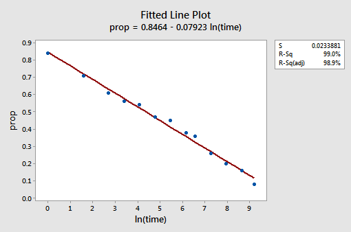
Indeed, the R2 value has increased from 57.1% to 99.0%. It tells us that 99% of the variation in the proportion of recalled words (prop) is reduced by taking into account the natural log of time (lntime)!
The new residual vs. fits plot shows a significant improvement over the one based on the untransformed data.
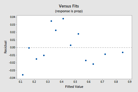
You might become concerned about some kind of a up-down cyclical trend in the plot. I caution you again not to over-interpret these plots, especially when the data set is small like this. You really shouldn't expect perfection when you resort to taking data transformations. Sometimes you have to just be content with significant improvements. By the way, the plot also suggests that it is okay to assume that the error variances are equal.
The normal probability plot of the residuals shows that transforming the x values had no effect on the normality of the error terms:

Again the Anderson-Darling P-value is large, so we fail to reject the null hypothesis of normal error terms. There is not enough evidence to conclude that the errors terms are not normal.
What if we had transformed the y values instead? Earlier I said that while some assumptions may appear to hold prior to applying a transformation, they may no longer hold once a transformation is applied. For example, if the error terms are well-behaved, transforming the y values could change them into badly-behaved error terms. The error terms for the memory retention data prior to transforming the x values appear to be well-behaved (in the sense that they appear approximately normal). Therefore, we might expect that transforming the y values instead of the x values could cause the error terms to become badly-behaved. Let's take a quick look at the memory retention data to see an example of what can happen when we transform the y values when non-linearity is the only problem.
By trial and error, we discover that the power transformation of y that does the best job at correcting the non-linearity is y-1.25. The fitted line plot illustrates that the transformation does indeed straighten out the relationship — although admittedly not as well as the log transformation of the x values.
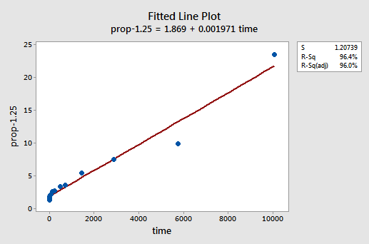
Note that the R2 value has increased from 57.1% to 96.4%.
The residuals show an improvement with respect to non-linearity, although the improvement is not great...
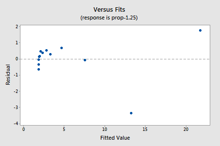
...but now we have non-normal error terms! The Anderson-Darling P-value is less than 0.005, so we reject the null hypothesis of normal error terms. There is sufficient evidence to conclude that the error terms are not normal:
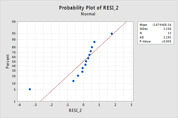
Again, if the error terms are well-behaved prior to transformation, transforming the y values can change them into badly-behaved error terms.
Using the model
Once we've found the best model for our regression data, we can then use the model to answer our research questions of interest. If our model involves transformed predictor (x) values, we may or may not have to make slight modifications to the standard procedures we've already learned.
Let's use our linear regression model for the memory retention data—with y = prop as the response and x = lntime as the predictor—to answer four different research questions.
Research Question #1: What is the nature of the association between time since memorized and the effectiveness of recall?
To answer this research question, we just describe the nature of the relationship. That is, the proportion of correctly recalled words is negatively linearly related to the natural log of the time since the words were memorized. Not surprisingly, as the natural log of time increases, the proportion of recalled words decreases.
Research Question #2: Is there an association between time since memorized and effectiveness of recall?
In answering this research question, no modification to the standard procedure is necessary. We merely test the null hypothesis H0: β1 = 0 using either the F-test or the equivalent t-test:
As the software output illustrates, the P-value is < 0.001. There is significant evidence at the 0.05 level to conclude that there is a linear association between the proportion of words recalled and the natural log of the time since memorized.
Research Question #3: What proportion of words can we expect a randomly selected person to recall after 1000 minutes?
We just need to calculate a prediction interval — with one slight modification — to answer this research question. Our predictor variable is the natural log of time. Therefore, when we use statistical software to calculate the prediction interval, we have to make sure that we specify the value of the predictor values in the transformed units, not the original units. The natural log of 1000 minutes is 6.91 log-minutes. Using software to calculate a 95% prediction interval when lntime = 6.91, we obtain:
The output tells us that we can be 95% confident that, after 1000 minutes, a randomly selected person will recall between 24.5% and 35.3% of the words.
Research Question #4: How much does the expected recall change if time increases ten-fold?
If you think about it, answering this research question merely involves estimating and interpreting the slope parameter β1. Well, not quite—there is a slight adjustment. In general, a k-fold increase in the predictor x is associated with a:
β1 × ln(k)
change in the mean of the response y.
This derivation that follows might help you understand and therefore remember this formula.
That is, a ten-fold increase in x is associated with a β1 × ln(10) change in the mean of y. And, a two-fold increase in x is associated with a β1 × ln(2) change in the mean of y.
In general, you should only use multiples of k that make sense for the scope of the model. For example, if the x values in your data set range from 2 to 8, it only makes sense to consider k multiples that are 4 or smaller. If the value of x were 2, a ten-fold increase (i.e., k = 10) would take you from 2 up to 2 × 10 = 20, a value outside the scope of the model. In the memory retention data set, the predictor values range from 1 to 10080, so there is no problem with considering a ten-fold increase.
If we are only interested in obtaining a point estimate, we merely take the estimate of the slope parameter (b1 = -0.079227) from the software output:
and multiply it by ln(10):
b1 × ln(10) = -0.079227 × ln(10) = -0.182
We expect the percentage of recalled words to decrease (since the sign is negative) 18.2% for each ten-fold increase in the time since memorization took place.
Of course, this point estimate is of limited usefulness. How confident can we be that the estimate is close to the true unknown value? Naturally, we should calculate a 95% confident interval. To do so, we just calculate a 95% confidence interval for β1 as we always have:
-0.079227 ± 2.201(0.002416) = (-0.085, -0.074)
and then multiply each endpoint of the interval by ln(10):
-0.074 × ln(10) = - 0.170 and -0.085 × ln(10) = - 0.l95
We can be 95% confident that the percentage of recalled words will decrease between 17.0% and 19.5% for each ten-fold increase in the time since memorization took place.

