7.6 - Interactions Between Quantitative Predictors
Interaction terms between quantitative predictors allow the relationship between the response and one predictor to vary with the values of another predictor. Interestingly, this provides another way to introduce curvature into a multiple linear regression model. For example, consider a model with two quantitative predictors, which we can visualize in a three-dimensional scatterplot with the response values placed vertically as usual and the predictors placed along the two horizontal axes. A multiple linear regression model with just these two predictors results in a flat fitted regression plane (like a flat piece of paper). If, however, we include an interaction between the predictors in our model, then the fitted regression plane looks like a piece of paper that has one edge sloped at one angle and the opposite edge sloped at a different angle, thus creating a three-dimensional curved plane.
Typically, regression models that include interactions between quantitative predictors adhere to the hierarchy principle, which says that if your model includes an interaction term, \(X_1X_2\), and \(X_1X_2\) is shown to be a statistically significant predictor of Y, then your model should also include the "main effects," \(X_1\) and \(X_2\), whether or not the coefficients for these main effects are significant. Depending on the subject area, there may be circumstances where a main effect could be excluded, but this tends to be the exception.
We can use interaction terms in any multiple linear regression model. Here we consider an example with two quantitative predictors and one indicator variable for a categorical predictor. In Lesson 5 we looked at some data resulting from a study in which the researchers (Colby, et al, 1987) wanted to determine if nestling bank swallows alter the way they breathe in order to survive the poor air quality conditions of their underground burrows. In reality, the researchers studied not only the breathing behavior of nestling bank swallows, but that of adult bank swallows as well.
To refresh your memory, the researchers conducted the following randomized experiment on 120 nestling bank swallows. In an underground burrow, they varied the percentage of oxygen at four different levels (13%, 15%, 17%, and 19%) and the percentage of carbon dioxide at five different levels (0%, 3%, 4.5%, 6%, and 9%). Under each of the resulting 5×4 = 20 experimental conditions, the researchers observed the total volume of air breathed per minute for each of 6 nestling bank swallows. They replicated the same randomized experiment on 120 adult bank swallows. In this way, they obtained the following data (allswallows.txt) on n = 240 swallows:
- Response (y): percentage increase in "minute ventilation", (Vent), i.e., total volume of air breathed per minute.
- Potential predictor (x1): percentage of oxygen (O2) in the air the swallows breathe
- Potential predictor (x2): percentage of carbon dioxide (CO2) in the air the swallows breathe
- Potential qualitative predictor (x3): (Type) 1 if bird is an adult, 0 if bird is a nestling
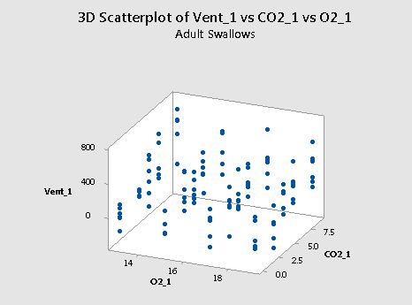
Here's a plot of the resulting data for the adult swallows:
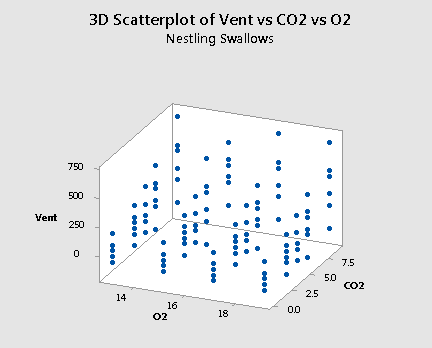
and a plot of the resulting data for the nestling bank swallows:
As mentioned previously, the "best fitting" function through each of the above plots will be some sort of surface like a sheet of paper. If you click on the Draw Plane button, you will see one possible estimate of the surface for the nestlings:
What we don't know is if the best fitting function —that is, the sheet of paper —through the data will be curved or not. Including interaction terms in the regression model allows the function to have some curvature, while leaving interaction terms out of the regression model forces the function to be flat.
Let's consider the research question "is there any evidence that the adults differ from the nestlings in terms of their minute ventilation as a function of oxygen and carbon dioxide?"
We could start by formulating the following multiple regression model with two quantitative predictors and one qualitative predictor:
\[y_i=(\beta_0+\beta_1x_{i1}+\beta_2x_{i2}+\beta_3x_{i3})+\epsilon_i\]
where:
- yi is the percentage of minute ventilation for swallow i
- xi1 is the percentage of oxygen for swallow i
- xi2 is the percentage of carbon dioxide for swallow i
- xi3 is the type of bird (0, if nestling and 1, if adult) for swallow i
and the independent error terms εi follow a normal distribution with mean 0 and equal variance σ2.
We now know, however, that there is a risk in omitting an important interaction term. Therefore, let's instead formulate the following multiple regression model with three interaction terms:
\[y_i=(\beta_0+\beta_1x_{i1}+\beta_2x_{i2}+\beta_3x_{i3}+\beta_{12}x_{i1}x_{i2}+\beta_{13}x_{i1}x_{i3}+\beta_{23}x_{i2}x_{i3})+\epsilon_i\]
where:
- yi is the percentage of minute ventilation for swallow i
- xi1 is the percentage of oxygen for swallow i
- xi2 is the percentage of carbon dioxide for swallow i
- xi3 is the type of bird (0, if nestling and 1, if adult) for swallow i
- xi1xi2, xi1xi3, and xi2xi3 are interaction terms
By setting the predictor x3 to equal 0 and 1 and doing a little bit of algebra we see that our formulated model yields two response functions —one for each type of bird:
| Type of bird | Formulated regression function |
| If a nestling, then xi3 = 0 and ... |
\(\mu_Y=\beta_0+\beta_1x_{i1}+\beta_2x_{i2}+\beta_{12}x_{i1}x_{i2}\) |
| If an adult, then xi3 = 1 and ... |
\(\mu_Y=(\beta_0+\beta_3)+(\beta_1+\beta_{13})x_{i1}+(\beta_2+\beta_{23})x_{i2}+\beta_{12}x_{i1}x_{i2}\) |
The β12xi1xi2 interaction term appearing in both functions allows the two functions to have the same curvature. The additional β13 parameter appearing before the xi1 predictor in the regression function for the adults allows the adult function to be shifted from the nestling function in the xi1 direction by β13 units. And, the additional β23 parameter appearing before the xi2 predictor in the regression function for the adults allows the adult function to be shifted from the nestling function in the xi2 direction by β23 units.
The results for this model are:
            Estimate Std. Error t value Pr(>|t|)
(Intercept)  -18.399    160.007  -0.115   0.9086
O2             1.189      9.854   0.121   0.9041
CO2           54.281     25.987   2.089   0.0378 *
Type         111.658    157.742   0.708   0.4797
TypeO2        -7.008      9.560  -0.733   0.4642
TypeCO2        2.311      7.126   0.324   0.7460
CO2O2         -1.449      1.593  -0.909   0.3642
---
Signif. codes:  0 ‘***’ 0.001 ‘**’ 0.01 ‘*’ 0.05 ‘.’ 0.1 ‘ ’ 1

Residual standard error: 165.6 on 233 degrees of freedom
Multiple R-squared:  0.272,	Adjusted R-squared:  0.2533
F-statistic: 14.51 on 6 and 233 DF,  p-value: 4.642e-14
Note that the P-values for each of the interaction parameters, β12, β13, and β23 are quite large, suggesting there is little evidence for two-way interactions between type of bird, oxygen level, and carbon dioxide level.
Again, however, we should minimize the number of hypothesis tests we perform—and thereby reduce the chance of committing Type I and Type II errors—by instead conducting a general linear F-test for testing H0: β12 = β13 = β23 = 0 simultaneously. The residual error sum of squares for this (full) model is 6,388,603 with 233 degrees of freedom. The residual error sum of squares for a (reduced) model that excludes the interaction terms is 6,428,886 with 236 degrees of freedom.
The general linear F-statistic is therefore:
\[F^*=\frac{(6428886-6388603)/3}{6388603/233}=0.49\]
And the following output:
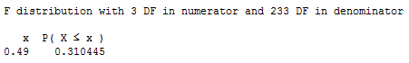
tells us that the probability of observing an F-statistic less than 0.49, with 3 numerator and 233 denominator degrees of freedom, is 0.31. Therefore, the probability of observing an F-statistic greater than 0.49, with 3 numerator and 233 denominator degrees of freedom, is 1-0.31 or 0.69. That is, the P-value is 0.69. There is insufficient evidence at the 0.05 level to conclude that at least one of the interaction parameters is not 0.
The residual versus fits plot:
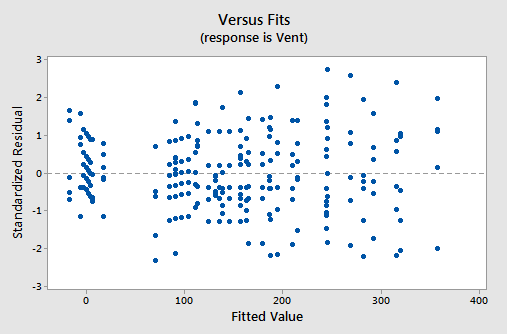
also suggests that there is something not quite right about the fit of the model containing interaction terms.
Incidentally, if we go back and re-examine the two scatter plots of the data —one for the adults:
and one for the nestlings:
we see that it is believable that there are no interaction terms. If you tried to "draw" the "best fitting" function through each scatter plot, the two functions would probably look like two parallel planes.
So, let's go back to formulating the model with no interactions terms:
\[y_i=(\beta_0+\beta_1x_{i1}+\beta_2x_{i2}+\beta_3x_{i3})+\epsilon_i\]
where:
- yi is the percentage of minute ventilation for swallow i
- xi1 is the percentage of oxygen for swallow i
- xi2 is the percentage of carbon dioxide for swallow i
- xi3 is the type of bird (0, if nestling and 1, if adult) for swallow i
and the independent error terms εi follow a normal distribution with mean 0 and equal variance σ2.
Using software to estimate the regression function, we obtain:
            Estimate Std. Error t value Pr(>|t|)
(Intercept)  136.767     79.334   1.724    0.086 .
O2            -8.834      4.765  -1.854    0.065 .
CO2           32.258      3.551   9.084   <2e-16 ***
Type           9.925     21.308   0.466    0.642
---
Signif. codes:  0 ‘***’ 0.001 ‘**’ 0.01 ‘*’ 0.05 ‘.’ 0.1 ‘ ’ 1

Residual standard error: 165 on 236 degrees of freedom
Multiple R-squared:  0.2675,	Adjusted R-squared:  0.2581
F-statistic: 28.72 on 3 and 236 DF,  p-value: 7.219e-16
Let's finally answer our primary research question: "is there any evidence that the adult swallows differ from the nestling swallows in terms of their minute ventilation as a function of oxygen and carbon dioxide?" To answer the question, we need only test the null hypothesis H0 : β3 = 0. The software output shows that the P-value is 0.642. We fail to reject the null hypothesis at any reasonable significance level. There is insufficient evidence to conclude that adult swallows differ from nestling swallows with respect to their minute ventilation.
Incidentally, before using the model to answer the research question, we should have assessed the model assumptions. All is fine, however. The residuals versus fits plot for the model with no interaction terms:
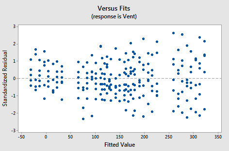
shows a marked improvement over the residuals versus fits plot for the model with the interaction terms. Perhaps there is a little bit of fanning? A little bit, but perhaps not enough to worry about.
And, the normal probability plot:
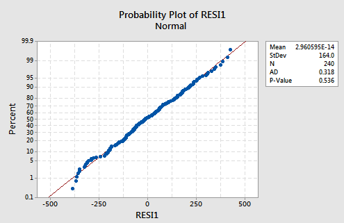
suggests there is no reason to worry about non-normal error terms.

