7.2 - Log-transforming Only the Response for SLR
In this section, we learn how to build and use a model by transforming the response y values. Transforming the y values should be considered when non-normality and/or unequal variances are the problems with the model. As an added bonus, the transformation on y may also help to "straighten out" a curved relationship.
Again, keep in mind that although we're focussing on a simple linear regression model here, the essential ideas apply more generally to multiple linear regression models too.
Building the model
An example. Let's consider data (mammgest.txt) on the typical birthweight and length of gestation for various mammals. We treat the birthweight (x, in kg) as the predictor and the length of gestation (y, in number of days until birth) as the response.
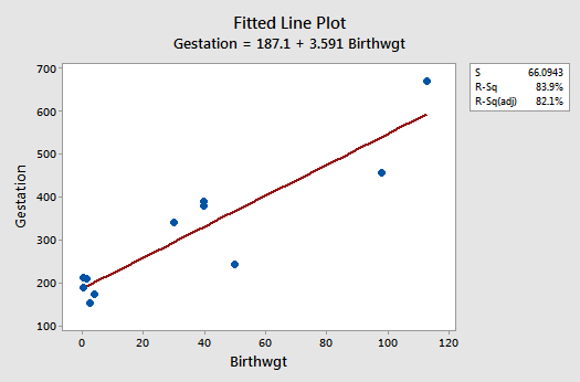
The fitted line plot suggests that the relationship between gestation length (y) and birthweight (x) is linear, but that the variance of the error terms might not be equal:
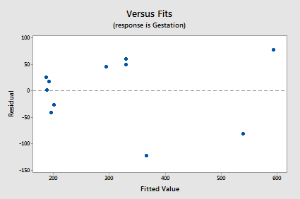
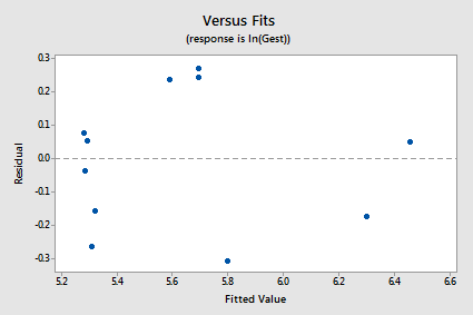
The residuals vs. fits plot exhibits some fanning and therefore provides yet more evidence that the variance of the error terms might not be equal:
The normal probability plot supports the assumption of normally distributed error terms:
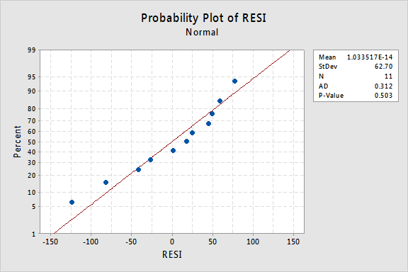
The line is approximately straight and the Anderson-Darling P-value is 0.503. We fail to reject the null hypothesis of normal error terms. There is not enough evidence to conclude that the errors terms are not normal.
Let's transform the y values by taking the natural logarithm of the lengths of gestation. Doing so, we obtain the new response y = lnGest:
| Mammal |
Birthwgt
|
Gestation
|
lnGest
|
| Goat |
2.75
|
155
|
5.04343
|
| Sheep |
4.00
|
175
|
5.16479
|
| Deer |
0.48
|
190
|
5.24702
|
| Porcupine |
1.50
|
210
|
5.34711
|
| Bear |
0.37
|
213
|
5.36129
|
| Hippo |
50.00
|
243
|
5.49306
|
| Horse |
30.00
|
340
|
5.82895
|
| Camel |
40.00
|
380
|
5.94017
|
| Zebra |
40.00
|
390
|
5.96615
|
| Giraffe |
98.00
|
457
|
6.12468
|
| Elephant |
113.00
|
670
|
6.50728
|
For example, ln(155) = 5.04343 and ln(457) = 6.12468. Now that we've transformed the response y values, let's see if it helped rectify the problem with the unequal error variances.
The fitted line plot with y = lnGest as the response and x = Birthwgt as the predictor suggests that the log transformation of the response has helped:
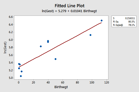
Note that, as expected, the log transformation has tended to "spread out" the smaller gestations and tended to "bring in" the larger ones.
The new residual vs. fits plot shows a marked improvement in the spread of the residuals:
The log transformation of the response did not adversely affect the normality of the error terms:
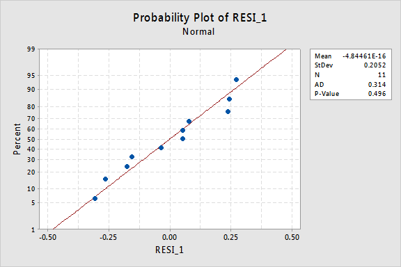
The line is approximately straight and the Anderson-Darling P-value is 0.496. We fail to reject the null hypothesis of normal error terms. There is not enough evidence to conclude that the errors terms are not normal.
Note that the R2 value is lower for the transformed model than for the untransformed model (80.3% versus 83.9%). This does not mean that the untransformed model is preferable. Remember the untransformed model failed to satisfy the equal variance condition, so we should not use this model anyway.
Again, transforming the y values should be considered when non-normality and/or unequal variances are the main problems with the model.
Using the model
We've identified what we think is the best model for the mammal birthweight and gestation data. The model meets the four "LINE" conditions. Therefore, we can use the model to answer our research questions of interest. We may or may not have to make slight modifications to the standard procedures we've already learned.
Let's use our linear regression model for the mammal birthweight and gestation data—with y = lnGest as the response and x = birthwgt as the predictor—to answer four different research questions.
Research Question #1: What is the nature of the association between mammalian birth weight and length of gestation?
Again, to answer this research question, we just describe the nature of the relationship. That is, the natural logarithm of the length of gestation is positively linearly related to birthweight. That is, as the average birthweight of the mammal increases, the expected natural logarithm of the gestation length also increases.
Research Question #2: Is there an association between mammalian birth weight and length of gestation?
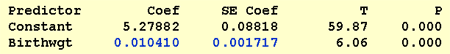
Again, in answering this research question, no modification to the standard procedure is necessary. We merely test the null hypothesis H0: β1 = 0 using either the F-test or the equivalent t-test:
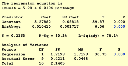
As the software output illustrates, the P-value is < 0.001. There is significant evidence at the 0.05 level to conclude that there is a linear association between the mammalian birthweight and the natural logarithm of the length of gestation.
Research Question #3: What is the expected gestation length of a new 50 kg mammal?
In answering this research question, if we are only interested in obtaining a point estimate, we merely enter x = 50 into the estimated regression equation:
\[ln(\widehat{Gest})=5.28+0.0104 \times Birthwgt\]
to obtain:
\[ln(\widehat{Gest})=5.28+0.0104 \times 50=5.8\]
That is, we predict the length of gestation of a 50 kg mammal to be 5.8 log-days! Well, that's not very informative! We need to transform the answer back into the original units. This just requires recalling one of the fundamental properties of the natural logarithm, namely that ex and ln(x) "cancel each other out." That is:
\[\widehat{Gest}=e^{ln(\widehat{Gest})}\]
Furthermore, if we exponentiate the left side of the equation:
\[ln(\widehat{Gest})=5.28+0.0104 \times 50=5.8\]
we also have to exponentiate the right side of the equation. Doing so, we obtain:
\[\widehat{Gest}=e^{ln(\widehat{Gest})}=e^{5.8}=330.3\]
We predict the gestation length of a 50 kg mammal to be 330 days. That sounds better!
Again, a point estimate is of limited usefulness. It doesn't tells us how confident we can be that the prediction is close to the true unknown value. We should calculate a 95% prediction interval:
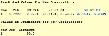
So, we can be 95% confident that the gestation length of a 50 kg mammal is predicted to be between 5.2847 and 6.3139 log-days! Again, we need to transform these predicted limits back into the original units. Doing so, we obtain:
e5.2847 = 197.3 and e6.3139 = 552.2
We can be 95% confident that the gestation length for a 50 kg mammal will be between 197.3 and 552.2 days.
Research Question #4: What is the expected change in length of gestation for each one pound increase in birth weight?
Figuring out how to answer this research question takes a little bit of work — and some creativity, too! If you only care about the end result, this is it:
- The median of the response changes by a factor of \(e^{\beta_1}\) for each one unit increase in the predictor x. Although you won't be required to duplicate the derivation, it might help you understand—and therefore remember—the result.
- And, therefore, the median of the response changes by a factor of \(e^{k\beta_1}\) for each k-unit increase in the predictor x. Again, although you won't be required to duplicate the derivation, it might help you understand—and therefore remember—the result.
- As always, we won't know the slope of the population line, β1, so we'll have to use b1 to estimate it.
For the mammalian birthweight and gestation data, the software output tells us that b1 = 0.01041:
and therefore:
\[e^{b_1}=e^{0.01041}=1.0105\]
The result tells us that the predicted median gestation changes by a factor of 1.0105 for each one unit increase in birthweight. For example, the predicted median gestation for a mammal weighing 3 kgs is 1.0105 times the median gestation for a mammal weighing 2 kgs. And, since there is a 10-unit increase going from a 20 kg to a 30 kg mammal, the median gestation for a mammal weighing 30 kgs is 1.010510 = 1.110 times the median gestation for a mammal weighing 20 kgs.
So far, we've only calculated a point estimate for the expected change. Of course, a 95% confidence interval for β1 is:
0.01041 ± 2.2622(0.001717) = (0.0065, 0.0143)
Because:
e0.0065 = 1.0065 and e0.0143 = 1.0144
we can be 95% confident that the median gestation will increase by a factor between 1.0065 and 1.0144 for each one kilogram increase in birth weight. And, since:
1.006510 = 1.067 and 1.014410 = 1.154
we can be 95% confident that the median gestation will increase by a factor between 1.067 and 1.154 for each 10-kilogram increase in birth weight.

