7.8 - Polynomial Regression Examples
Example 1: How is the length of a bluegill fish related to its age?
In 1981, n = 78 bluegills were randomly sampled from Lake Mary in Minnesota. The researchers (Cook and Weisberg, 1999) measured and recorded the following data (bluegills.txt):
- Response (y): length (in mm) of the fish
- Potential predictor (x1): age (in years) of the fish
The researchers were primarily interested in learning how the length of a bluegill fish is related to it age.
A scatter plot of the data:
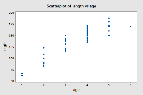
suggests that there is positive trend in the data. That is, not surprisingly, as the age of bluegill fish increases, the length of the fish tends to increase. The trend, however, doesn't appear to be quite linear. It appears as if the relationship is slightly curved.
One way of modeling the curvature in these data is to formulate a "second-order polynomial model" with one quantitative predictor:
\[y_i=(\beta_0+\beta_1x_{i}+\beta_{11}x_{i}^2)+\epsilon_i\]
where:
- yi is length of bluegill (fish) i (in mm)
- xi is age of bluegill (fish) i (in years)
and the independent error terms εi follow a normal distribution with mean 0 and equal variance σ2.
You may recall from your previous studies that "quadratic function" is another name for our formulated regression function. Nonetheless, you'll often hear statisticians referring to this quadratic model as a second-order model, because the highest power on the xi term is 2.
Incidentally, observe the notation used. Because there is only one predictor variable to keep track of, the 1 in the subscript of xi1 has been dropped. That is, we use our original notation of just xi. Also note the double subscript used on the slope term, β11, of the quadratic term, as a way of denoting that it is associated with the squared term of the one and only predictor.
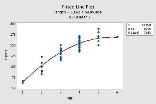
The estimated quadratic regression function looks like it does a pretty good job of fitting the data:
To answer the following potential research questions, do the procedures identified in parentheses seem reasonable?
- How is the length of a bluegill fish related to its age? (Describe the nature—"quadratic"—of the regression function.)
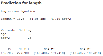
- What is the length of a randomly selected five-year-old bluegill fish? (Calculate and interpret a prediction interval for the response.)
Statistical software output follows:
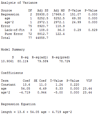
The output tells us that:
- 80.1% of the variation in the length of bluegill fish is reduced by taking into account a quadratic function of the age of the fish.
- We can be 95% confident that the length of a randomly selected five-year-old bluegill fish is between 143.5 and 188.3 mm.
 Example 2: Yield Data Set
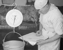
This data set of size n = 15 (yield.txt) contains measurements of yield from an experiment done at five different temperature levels. The variables are y = yield and x = temperature in degrees Fahrenheit. The table below gives the data used for this analysis.
| i | Temperature | Yield |
| 1 | 50 | 3.3 |
| 2 | 50 | 2.8 |
| 3 | 50 | 2.9 |
| 4 | 70 | 2.3 |
| 5 | 70 | 2.6 |
| 6 | 70 | 2.1 |
| 7 | 80 | 2.5 |
| 8 | 80 | 2.9 |
| 9 | 80 | 2.4 |
| 10 | 90 | 3.0 |
| 11 | 90 | 3.1 |
| 12 | 90 | 2.8 |
| 13 | 100 | 3.3 |
| 14 | 100 | 3.5 |
| 15 | 100 | 3.0 |
The figures below give a scatterplot of the raw data and then another scatterplot with lines pertaining to a linear fit and a quadratic fit overlayed. Obviously the trend of this data is better suited to a quadratic fit.
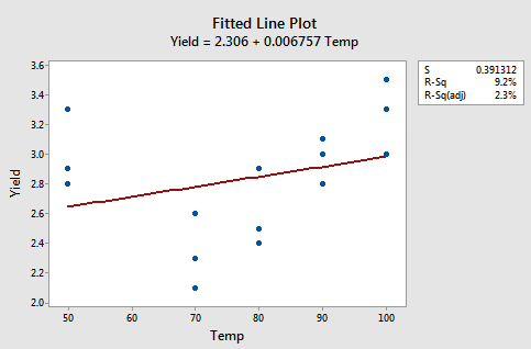
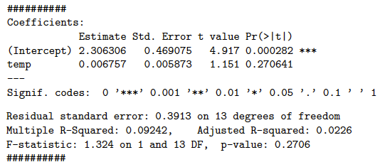
Here we have the linear fit results:
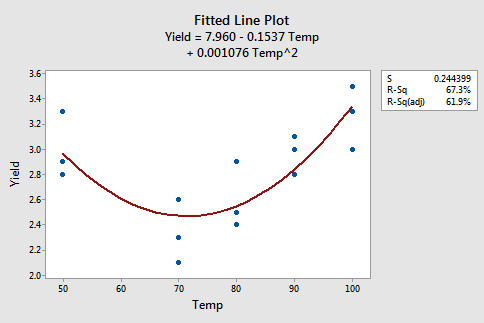
Here we have the quadratic fit results:
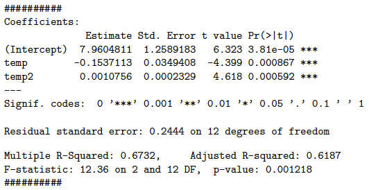
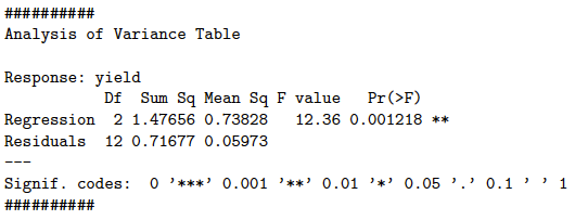
We see that both temperature and temperature squared are significant predictors for the quadratic model (with p-values of 0.0009 and 0.0006, respectively) and that the fit is much better than for the linear fit. From this output, we see the estimated regression equation is \(y_{i}=7.96050-0.15371x_{i}+0.00108x_{i}^{2}\). Furthermore, the ANOVA table below shows that the model we fit is statistically significant at the 0.05 significance level with a p-value of 0.0012. Thus, our model should include a quadratic term.
 Example 3: Odor Data Set
An experiment is designed to relate three variables (temperature, ratio, and height) to a measure of odor in a chemical process. Each variable has three levels, but the design was not constructed as a full factorial design (i.e., it is not a \(3^{3}\) design). Nonetheless, we can still analyze the data using a response surface regression routine, which is essentially polynomial regression with multiple predictors. The data obtained (odor.txt) was already coded and can be found in the table below.
| Odor | Temperature | Ratio | Height |
| 66 | -1 | -1 | 0 |
| 58 | -1 | 0 | -1 |
| 65 | 0 | -1 | -1 |
| -31 | 0 | 0 | 0 |
| 39 | 1 | -1 | 0 |
| 17 | 1 | 0 | -1 |
| 7 | 0 | 1 | -1 |
| -35 | 0 | 0 | 0 |
| 43 | -1 | 1 | 0 |
| -5 | -1 | 0 | 1 |
| 43 | 0 | -1 | 1 |
| -26 | 0 | 0 | 0 |
| 49 | 1 | 1 | 0 |
| -40 | 1 | 0 | 1 |
| -22 | 0 | 1 | 1 |
First we will fit a response surface regression model consisting of all of the first-order and second-order terms. The summary of this fit is given below:
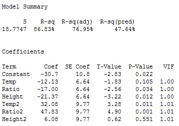
As you can see, the square of height is the least statistically significant, so we will drop that term and rerun the analysis. The summary of this new fit is given below:
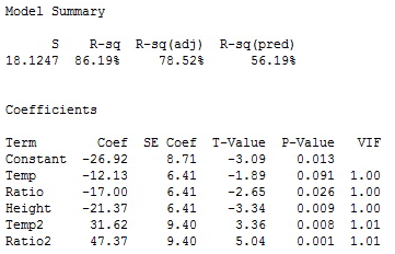
The temperature main effect (i.e., the first-order temperature term) is not significant at the usual 0.05 significance level. However, the square of temperature is statistically significant. To adhere to the hierarchy principle, we retain the temperature main effect in the model.

