Lesson 5: Multiple Linear Regression
Lesson 5: Multiple Linear RegressionOverview
In this lesson, we make our first (and last?!) major jump in the course. We move from the simple linear regression model with one predictor to the multiple linear regression model with two or more predictors. That is, we use the adjective "simple" to denote that our model has only predictors, and we use the adjective "multiple" to indicate that our model has at least two predictors.
In the multiple regression setting, because of the potentially large number of predictors, it is more efficient to use matrices to define the regression model and the subsequent analyses. This lesson considers some of the more important multiple regression formulas in matrix form. If you're unsure about any of this, it may be a good time to take a look at this Matrix Algebra Review.
The good news!
The good news is that everything you learned about the simple linear regression model extends — with at most minor modifications — to the multiple linear regression model. Think about it — you don't have to forget all of that good stuff you learned! In particular:
- The models have similar "LINE" assumptions. The only real difference is that whereas in simple linear regression we think of the distribution of errors at a fixed value of the single predictor, with multiple linear regression we have to think of the distribution of errors at a fixed set of values for all the predictors. All of the model-checking procedures we learned earlier are useful in the multiple linear regression framework, although the process becomes more involved since we now have multiple predictors. We'll explore this issue further in Lesson 7.
- The use and interpretation of \(R^2\) in the context of multiple linear regression remains the same. However, with multiple linear regression, we can also make use of an "adjusted" \(R^2\) value, which is useful for model-building purposes. We'll explore this measure further in Lesson 10.
- With a minor generalization of the degrees of freedom, we use t-tests and t-intervals for the regression slope coefficients to assess whether a predictor is significantly linearly related to the response, after controlling for the effects of all the other predictors in the model.
- With a minor generalization of the degrees of freedom, we use prediction intervals for predicting an individual response and confidence intervals for estimating the mean response. We'll explore these further in Lesson 7.
Objectives
- Know how to calculate a confidence interval for a single slope parameter in the multiple regression setting.
- Be able to interpret the coefficients of a multiple regression model.
- Understand what the scope of the model is in the multiple regression model.
- Understand the calculation and interpretation of R2 in a multiple regression setting.
- Understand the calculation and use of adjusted R2 in a multiple regression setting.
Lesson 5 Code Files
Below is a zip file that contains all the data sets used in this lesson:
- babybirds.txt
- bodyfat.txt
- hospital_infct.txt
- fev_dat.txt
- iqsize.txt
- pastry.txt
- soapsuds.txt
- stat_females.txt
5.1 - Example on IQ and Physical Characteristics
5.1 - Example on IQ and Physical CharacteristicsExample 5-1
Let's jump in and take a look at some "real-life" examples in which a multiple linear regression model is used. Make sure you notice, in each case, that the model has more than one predictor. You might also try to pay attention to the similarities and differences among the examples and their resulting models. Most of all, don't worry about mastering all of the details now. In the upcoming lessons, we will revisit similar examples in greater detail. For now, my hope is that these examples leave you with an appreciation of the richness of multiple regression.
Are a person's brain size and body size predictive of his or her intelligence?
Interested in answering the above research question, some researchers (Willerman, et al, 1991) collected the following data (IQ Size data) on a sample of n = 38 college students:
- Response (y): Performance IQ scores (PIQ) from the revised Wechsler Adult Intelligence Scale. This variable served as the investigator's measure of the individual's intelligence.
- Potential predictor (\(x_{1}\)): Brain size based on the count obtained from MRI scans (given as count/10,000).
- Potential predictor (\(x_{2}\)): Height in inches.
- Potential predictor (\(x_{3}\)): Weight in pounds.
As always, the first thing we should want to do when presented with a set of data is to plot it. And, of course, plotting the data is a little more challenging in the multiple regression setting, as there is one scatter plot for each pair of variables. Not only do we have to consider the relationship between the response and each of the predictors, but we also have to consider how the predictors are related to each other.
A common way of investigating the relationships among all of the variables is by way of a "scatter plot matrix." Basically, a scatter plot matrix contains a scatter plot of each pair of variables arranged in an orderly array. Here's what one version of a scatter plot matrix looks like for our brain and body size example:
For each scatterplot in the matrix, the variable on the y-axis appears at the left end of the plot's row and the variable on the x-axis appears at the bottom of the plot's column. Try to identify the variables on the y-axis and x-axis in each of the six scatter plots appearing in the matrix. You can check your understanding by selecting the icons appearing in the above matrix.
Incidentally, in case you are wondering, the tick marks on each of the axes are located at 25%, and 75% of the data range from the minimum. That is:
- the first tick = ((maximum - minimum) * 0.25) + minimum
- the second tick = ((maximum - minimum) * 0.75) + minimum
Now, what does a scatterplot matrix tell us? Of course, one use of the plots is simple data checking. Are there any egregiously erroneous data errors? The scatter plots also illustrate the "marginal relationships" between each pair of variables without regard to the other variables. For example, it appears that brain size is the best single predictor of PIQ, but none of the relationships are particularly strong. In multiple linear regression, the challenge is to see how the response y relates to all three predictors simultaneously.
We always start a regression analysis by formulating a model for our data. One possible multiple linear regression model with three quantitative predictors for our brain and body size example is:
\(y_i=(\beta_0+\beta_1x_{i1}+\beta_2x_{i2}+\beta_3x_{i3})+\epsilon_i\)
where:
- \(y_{i}\) is the intelligence (PIQ) of student i
- \(x_{i1}\) is the brain size (MRI) of student i
- \(x_{i2}\) is the height (Height) of student i
- \(x_{i3}\) is the weight (Weight) of student i
and the independent error terms \(\epsilon_{i}\) follow a normal distribution with mean 0 and equal variance \(\sigma_{2}\).
A couple of things to note about this model:
- Because we have more than one predictor (x) variable, we use slightly modified notation. The x-variables (e.g., \(x_{i1}\), \(x_{i2}\), and \(x_{i3}\)) are now subscripted with a 1, 2, and 3 as a way of keeping track of the three different quantitative variables. We also subscript the slope parameters with the corresponding numbers (e.g., \(\beta_{1}\) \(\beta_{2}\) and \(\beta_{3}\)).
- The "LINE" conditions must still hold for the multiple linear regression model. The linear part comes from the formulated regression function — it is, what we say, "linear in the parameters." This simply means that each beta coefficient multiplies a predictor variable or a transformation of one or more predictor variables. We'll see in Lesson 9 that this means that, for example, the model, \(y=\beta_0+\beta_1x+\beta_2x^2+\epsilon\), is a multiple linear regression model even though it represents a curved relationship between \(y\) and \(x\).
Of course, our interest in performing a regression analysis is almost always to answer some sort of research question. Can you think of some research questions that the researchers might want to answer here? How about the following set of questions? What procedure would you use to answer each research question? (Do the procedures that appear in parentheses seem reasonable?)
- Which, if any, predictors — brain size, height, or weight — explain some of the variations in intelligence scores? (Conduct hypothesis tests for individually testing whether each slope parameter could be 0.)
- What is the effect of brain size on PIQ, after taking into account height and weight? (Calculate and interpret a confidence interval for the brain size slope parameter.)
- What is the PIQ of an individual with given brain size, height, and weight? (Calculate and interpret a prediction interval for the response.)
Let's take a look at the output we obtain when we ask Minitab to estimate the multiple regression model we formulated above:
Regression Analysis: PIQ versus Brain, Height, Weight
Analysis of Variance
| Source | DF | Adj SS | Adj MS | F-Value | P-value |
|---|---|---|---|---|---|
| Regression | 3 | 5572.7 | 1857.58 | 4.74 | 0.007 |
| Brain | 1 | 5239.2 | 5239.23 | 13.37 | 0.001 |
| Height | 1 | 1934.7 | 1934.71 | 4.94 | 0.033 |
| Weight | 1 | 0.0 | 0.0 | 0.00 | 0.998 |
| Error | 34 | 13321.8 | 391.82 | ||
| Total | 37 | 188946 |
Model Summary
| S | R-sq | R-sq(adj) | R-sq(pred) |
|---|---|---|---|
| 19.7944 | 29.49% | 23.27% | 12.76% |
Coefficients
| Term | Coef | SE Coef | T-Value | P-Value | VIF |
|---|---|---|---|---|---|
| Constant | 11.4 | 63.0 | 1.77 | 0.086 | |
| Brain | 2.060 | 0.563 | 3.66 | 0.001 | 1.58 |
| Height | -2.73 | 1.23 | -2.22 | 0.033 | 2.28 |
| Weight | 0.001 | 0.197 | 0.00 | 0.998 | 2.02 |
Regression Equation
PIQ = 111.4 + 2.060 Brain - 2.73 Height + 0.001 Weight
My hope is that you immediately observe that much of the output looks the same as before! The only substantial differences are:
- More predictors appear in the estimated regression equation and therefore also in the column labeled "Term" in the coefficients table.
- There is an additional row for each predictor term in the Analysis of Variance Table. By default in Minitab, these represent the reductions in the error sum of squares for each term relative to a model that contains all of the remaining terms (so-called Adjusted or Type III sums of squares). It is possible to change this using the Minitab Regression Options to instead use Sequential or Type I sums of squares, which represent the reductions in error sum of squares when a term is added to a model that contains only the terms before it.
We'll learn more about these differences later, but let's focus now on what you already know. The output tells us that:
- The \(R^{2}\) value is 29.49%. This tells us that 29.49% of the variation in intelligence, as quantified by PIQ, is reduced by taking into account brain size, height, and weight.
- The Adjusted \(R^{2}\) value — denoted "R-sq(adj)" — is 23.27%. When considering different multiple linear regression models for PIQ, we could use this value to help compare the models.
- The P-values for the t-tests appearing in the coefficients table suggest that the slope parameters for Brain (P = 0.001) and Height (P = 0.033) are significantly different from 0, while the slope parameter for Weight (P = 0.998) is not.
- The P-value for the analysis of variance F-test (P = 0.007) suggests that the model containing Brain, Height, and Weight is more useful in predicting intelligence than not taking into account the three predictors. (Note that this does not tell us that the model with the three predictors is the best model!)
So, we already have a pretty good start on this multiple linear regression stuff. Let's take a look at another example.
5.2 - Example on Underground Air Quality
5.2 - Example on Underground Air QualityExampe 5-2: What are the breathing habits of baby birds that live in underground burrows?

Some mammals burrow into the ground to live. Scientists have found that the quality of the air in these burrows is not as good as the air aboveground. In fact, some mammals change the way that they breathe in order to accommodate living in poor air quality conditions underground.
Some researchers (Colby, et al, 1987) wanted to find out if nestling bank swallows, which live in underground burrows, also alter how they breathe. The researchers conducted a randomized experiment on n = 120 nestling bank swallows. In an underground burrow, they varied the percentage of oxygen at four different levels (13%, 15%, 17%, and 19%) and the percentage of carbon dioxide at five different levels (0%, 3%, 4.5%, 6%, and 9%). Under each of the resulting 5 × 4 = 20 experimental conditions, the researchers observed the total volume of air breathed per minute for each of 6 nestling bank swallows. In this way, they obtained the following data (Baby birds) on the n = 120 nestling bank swallows:
- Response (y): percentage increase in "minute ventilation," (Vent), i.e., the total volume of air breathed per minute.
- Potential predictor (\(x_{1}\)): percentage of oxygen (O2) in the air the baby birds breathe.
- Potential predictor (\(x_{2}\)): percentage of carbon dioxide (CO2) in the air the baby birds breathe.
Here's a scatter plot matrix of the resulting data obtained by the researchers:
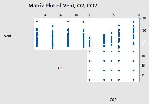
What does this particular scatter plot matrix tell us? Do you buy into the following statements?
- There doesn't appear to be a substantial relationship between minute ventilation (Vent) and the percentage of oxygen (O2).
- The relationship between minute ventilation (Vent) and the percentage of carbon dioxide (CO2) appears to be curved and with increasing error variance.
- The plot between the percentage of oxygen (O2) and the percentage of carbon dioxide (CO2) is the classical appearance of a scatter plot for the experimental conditions. The plot suggests that there is no correlation at all between the two variables. You should be able to observe from the plot the 4 levels of O2 and the 5 levels of CO2 that make up the 5×4 = 20 experimental conditions.
When we have one response variable and only two predictor variables, we have another sometimes useful plot at our disposal, namely a "three-dimensional scatter plot:"
If we added the estimated regression equation to the plot, what one word do you think describes what it would look like? Drag the slider on the bottom of the graph above to show the plot of the estimated regression equation for this data. Does it make sense that it looks like a "plane?" Incidentally, it is still important to remember that the plane depicted in the plot is just an estimate of the actual plane in the population that we are trying to study.
Here is a reasonable "first-order" model with two quantitative predictors that we could consider when trying to summarize the trend in the data:
\(y_i=(\beta_0+\beta_1x_{i1}+\beta_2x_{i2})+\epsilon_i\)
where:
- \(y_{i}\) is the percentage of minute ventilation of nestling bank swallow i
- \(x_{i1}\) is the percentage of oxygen exposed to nestling bank swallow i
- \(x_{i2}\) is the percentage of carbon dioxide exposed to nestling bank swallow i
and the independent error terms \(\epsilon_i\) follow a normal distribution with mean 0 and equal variance \(\sigma^{2}\).
The adjective "first-order" is used to characterize a model in which the highest power on all of the predictor terms is one. In this case, the power on \(x_{i1}\), although typically not shown, is one. And, the power on \(x_{i2}\) is also one, although not shown. Therefore, the model we formulated can be classified as a "first-order model." An example of a second-order model would be \(y=\beta_0+\beta_1x+\beta_2x^2+\epsilon\).
Do you have your research questions ready? How about the following set of questions? (Do the procedures that appear in parentheses seem appropriate in answering the research question?)
- Is oxygen related to minute ventilation, after taking into account carbon dioxide? (Conduct a hypothesis test for testing whether the O2 slope parameter is 0.)
- Is carbon dioxide related to minute ventilation, after taking into account oxygen? (Conduct a hypothesis test for testing whether the CO2 slope parameter is 0.)
- What is the mean minute ventilation of all nestling bank swallows whose breathing air is comprised of 15% oxygen and 5% carbon dioxide? (Calculate and interpret a confidence interval for the mean response.)
Here's the output we obtain when we ask Minitab to estimate the multiple regression model we formulated above:
Regression Analysis: Vent versus O2, CO2
| Source | DF | Adj SS | Adj MS | F-Value | P-value |
|---|---|---|---|---|---|
| Regression | 2 | 1061819 | 530909 | 21.44 | 0.000 |
| O2 | 1 | 17045 | 17045 | 0.69 | 0.408 |
| CO2 | 1 | 1044773 | 1044773 | 42.19 | 0.000 |
| Error | 117 | 2897566 | 24766 | ||
| Lack-of-Fit | 17 | 91284 | 5370 | 0.19 | 1.000 |
| Pure Error | 100 | 205172 | 18063 | ||
| Total | 119 | 3959385 |
| S | R-sq | R-sq(adj) | R-sq(pred) |
|---|---|---|---|
| 157.371 | 26.82% | 25.57% | 22.78% |
| Term | Coef | SE Coef | T-Value | P-Value | VIF |
|---|---|---|---|---|---|
| Constant | 86 | 106 | 0.81 | 0.419 | |
| O2 | -5.33 | 6.42 | -0.83 | 0.408 | 1.00 |
| CO2 | 31.10 | 4.79 | 6.50 | 0.000 |
1.00 |
Regression Equation
Vent = 86 - 5.33 O2 + 31.10 CO2
What do we learn from the Minitab output?
- Only 26.82% of the variation in minute ventilation is reduced by taking into account the percentages of oxygen and carbon dioxide.
- The P-values for the t-tests appearing in the coefficients table suggest that the slope parameter for carbon dioxide level (P < 0.001) is significantly different from 0, while the slope parameter for oxygen level (P = 0.408) is not. Does this conclusion appear consistent with the above scatter plot matrix and the three-dimensional plot? Yes!
- The P-value for the analysis of variance F-test (P < 0.001) suggests that the model containing oxygen and carbon dioxide levels is more useful in predicting minute ventilation than not taking into account the two predictors. (Again, the F-test does not tell us that the model with the two predictors is the best model! For one thing, we have performed no model checking yet!)
5.3 - The Multiple Linear Regression Model
5.3 - The Multiple Linear Regression ModelNotation for the Population Model
- A population model for a multiple linear regression model that relates a y-variable to p -1 x-variables is written as
\(\begin{equation} y_{i}=\beta_{0}+\beta_{1}x_{i,1}+\beta_{2}x_{i,2}+\ldots+\beta_{p-1}x_{i,p-1}+\epsilon_{i}. \end{equation} \)
- We assume that the \(\epsilon_{i}\) have a normal distribution with mean 0 and constant variance \(\sigma^{2}\). These are the same assumptions that we used in simple regression with one x-variable.
- The subscript i refers to the \(i^{\textrm{th}}\) individual or unit in the population. In the notation for the x-variables, the subscript following i simply denotes which x-variable it is.
- The word "linear" in "multiple linear regression" refers to the fact that the model is linear in the parameters, \(\beta_0, \beta_1, \ldots, \beta_{p-1}\). This simply means that each parameter multiplies an x-variable, while the regression function is a sum of these "parameter times x-variable" terms. Each x-variable can be a predictor variable or a transformation of predictor variables (such as the square of a predictor variable or two predictor variables multiplied together). Allowing non-linear transformation of predictor variables like this enables the multiple linear regression model to represent non-linear relationships between the response variable and the predictor variables. We'll explore predictor transformations further in Lesson 9. Note that even \(\beta_0\) represents a "parameter times x-variable" term if you think of the x-variable that is multiplied by \(\beta_0\) as being the constant function "1."
- The model includes p-1 x-variables, but p regression parameters (beta) because of the intercept term \(\beta_0\).
Estimates of the Model Parameters
- The estimates of the \(\beta\) parameters are the values that minimize the sum of squared errors for the sample. The exact formula for this is given in the next section on matrix notation.
- The letter b is used to represent a sample estimate of a \(\beta\) parameter. Thus \(b_{0}\) is the sample estimate of \(\beta_{0}\), \(b_{1}\) is the sample estimate of \(\beta_{1}\), and so on.
- \(\textrm{MSE}=\frac{\textrm{SSE}}{n-p}\) estimates \(\sigma^{2}\), the variance of the errors. In the formula, n = sample size, p = number of \(\beta\) parameters in the model (including the intercept) and \(\textrm{SSE}\) = sum of squared errors. Notice that for simple linear regression p = 2. Thus, we get the formula for MSE that we introduced in the context of one predictor.
- \(S=\sqrt{MSE}\) estimates \(\sigma\) and is known as the regression standard error or the residual standard error.
- In the case of two predictors, the estimated regression equation yields a plane (as opposed to a line in the simple linear regression setting). For more than two predictors, the estimated regression equation yields a hyperplane.
Interpretation of the Model Parameters
- Each \(\beta\) parameter represents the change in the mean response, E(y), per unit increase in the associated predictor variable when all the other predictors are held constant.
- For example, \(\beta_1\) represents the estimated change in the mean response, E(y), per unit increase in \(x_1\) when \(x_2\), \(x_3\), ..., \(x_{p-1}\) are held constant.
- The intercept term, \(\beta_0\), represents the estimated mean response, E(y), when all the predictors \(x_1\), \(x_2\), ..., \(x_{p-1}\), are all zero (which may or may not have any practical meaning).
Predicted Values and Residuals
- A predicted value is calculated as \(\hat{y}_{i}=b_{0}+b_{1}x_{i,1}+b_{2}x_{i,2}+\ldots+b_{p-1}x_{i,p-1}\), where the b values come from statistical software and the x-values are specified by us.
- A residual (error) term is calculated as \(e_{i}=y_{i}-\hat{y}_{i}\), the difference between an actual and a predicted value of y.
- A plot of residuals (vertical) versus predicted values (horizontal) ideally should resemble a horizontal random band. Departures from this form indicate difficulties with the model and/or data.
- Other residual analyses can be done exactly as we did in simple regression. For instance, we might wish to examine a normal probability plot (NPP) of the residuals. Additional plots to consider are plots of residuals versus each x-variable separately. This might help us identify sources of curvature or nonconstant variance. We'll explore this further in Lesson 7.
ANOVA Table
| Source | df | SS | MS | F |
|---|---|---|---|---|
| Regression | p – 1 | SSR | MSR = SSR / (p – 1) | MSR / MSE |
| Error | n – p | SSE | MSE = SSE / (n – p) | |
| Total | n – 1 | SSTO |
Coefficient of Determination, R-squared, and Adjusted R-squared
- As in simple linear regression, \(R^2=\frac{SSR}{SSTO}=1-\frac{SSE}{SSTO}\), and represents the proportion of variation in \(y\) (about its mean) "explained" by the multiple linear regression model with predictors, \(x_1, x_2, ...\).
- If we start with a simple linear regression model with one predictor variable, \(x_1\), then add a second predictor variable, \(x_2\), \(SSE\) will decrease (or stay the same) while \(SSTO\) remains constant, and so \(R^2\) will increase (or stay the same). In other words, \(R^2\) always increases (or stays the same) as more predictors are added to a multiple linear regression model, even if the predictors added are unrelated to the response variable. Thus, by itself, \(R^2\) cannot be used to help us identify which predictors should be included in a model and which should be excluded.
- An alternative measure, adjusted \(R^2\), does not necessarily increase as more predictors are added, and can be used to help us identify which predictors should be included in a model and which should be excluded. Adjusted \(R^2=1-\left(\frac{n-1}{n-p}\right)(1-R^2)\), and, while it has no practical interpretation, is useful for such model building purposes. Simply stated, when comparing two models used to predict the same response variable, we generally prefer the model with the higher value of adjusted \(R^2\) – see Lesson 10 for more details.
Significance Testing of Each Variable
Within a multiple regression model, we may want to know whether a particular x-variable is making a useful contribution to the model. That is, given the presence of the other x-variables in the model, does a particular x-variable help us predict or explain the y-variable? For instance, suppose that we have three x-variables in the model. The general structure of the model could be
\(\begin{equation} y=\beta _{0}+\beta _{1}x_{1}+\beta_{2}x_{2}+\beta_{3}x_{3}+\epsilon. \end{equation}\)
As an example, to determine whether variable \(x_{1}\) is a useful predictor variable in this model, we could test
\(\begin{align*} \nonumber H_{0}&\colon\beta_{1}=0 \\ \nonumber H_{A}&\colon\beta_{1}\neq 0 \end{align*}\)
If the null hypothesis above were the case, then a change in the value of \(x_{1}\) would not change y, so y and \(x_{1}\) are not linearly related (taking into account \(x_2\) and \(x_3\)). Also, we would still be left with variables \(x_{2}\) and \(x_{3}\) being present in the model. When we cannot reject the null hypothesis above, we should say that we do not need variable \(x_{1}\) in the model given that variables \(x_{2}\) and \(x_{3}\) will remain in the model. In general, the interpretation of a slope in multiple regression can be tricky. Correlations among the predictors can change the slope values dramatically from what they would be in separate simple regressions.
To carry out the test, statistical software will report p-values for all coefficients in the model. Each p-value will be based on a t-statistic calculated as
\(t^{*}=\dfrac{ (\text{sample coefficient} - \text{hypothesized value})}{\text{standard error of coefficient}}\)
For our example above, the t-statistic is:
\(\begin{equation*} t^{*}=\dfrac{b_{1}-0}{\textrm{se}(b_{1})}=\dfrac{b_{1}}{\textrm{se}(b_{1})}. \end{equation*}\)
Note that the hypothesized value is usually just 0, so this portion of the formula is often omitted.
Multiple linear regression, in contrast to simple linear regression, involves multiple predictors and so testing each variable can quickly become complicated. For example, suppose we apply two separate tests for two predictors, say \(x_1\) and \(x_2\), and both tests have high p-values. One test suggests \(x_1\) is not needed in a model with all the other predictors included, while the other test suggests \(x_2\) is not needed in a model with all the other predictors included. But, this doesn't necessarily mean that both \(x_1\) and \(x_2\) are not needed in a model with all the other predictors included. It may well turn out that we would do better to omit either \(x_1\) or \(x_2\) from the model, but not both. How then do we determine what to do? We'll explore this issue further in Lesson 6.
5.4 - A Matrix Formulation of the Multiple Regression Model
5.4 - A Matrix Formulation of the Multiple Regression ModelA matrix formulation of the multiple regression model
In the multiple regression setting, because of the potentially large number of predictors, it is more efficient to use matrices to define the regression model and the subsequent analyses. Here, we review basic matrix algebra, as well as learn some of the more important multiple regression formulas in matrix form.
As always, let's start with the simple case first. Consider the following simple linear regression function:
\(y_i=\beta_0+\beta_1x_i+\epsilon_i \;\;\;\;\;\;\; \text {for } i=1, ... , n\)
If we actually let i = 1, ..., n, we see that we obtain n equations:
\(\begin{align}
y_1 & =\beta_0+\beta_1x_1+\epsilon_1 \\
y_2 & =\beta_0+\beta_1x_2+\epsilon_2 \\
\vdots \\
y_n & = \beta_0+\beta_1x_n+\epsilon_n
\end{align}\)
Well, that's a pretty inefficient way of writing it all out! As you can see, there is a pattern that emerges. By taking advantage of this pattern, we can instead formulate the above simple linear regression function in matrix notation:
\(\underbrace{\vphantom{\begin{bmatrix}
1 & x_1\\
1 & x_2\\
\vdots &\vdots\\1&x_n
\end{bmatrix}}\begin{bmatrix}
y_1\\
y_2\\
\vdots\\y_n
\end{bmatrix}}_{\textstyle \begin{gathered}Y\end{gathered}}=\underbrace{\begin{bmatrix}
1 & x_1\\
1 & x_2\\
\vdots &\vdots\\1&x_n
\end{bmatrix}}_{\textstyle \begin{gathered}=X\end{gathered}} \underbrace{\vphantom{\begin{bmatrix}
1 & x_1\\
1 & x_2\\
\vdots &\vdots\\1&x_n
\end{bmatrix}}\begin{bmatrix}
\beta_0 \\
\beta_1\\
\end{bmatrix}}_{\textstyle \begin{gathered}\beta\end{gathered}}+\underbrace{\vphantom{\begin{bmatrix}
1 & x_1\\
1 & x_2\\
\vdots &\vdots\\1&x_n
\end{bmatrix}}\begin{bmatrix}\epsilon_1\\\epsilon_2\\\vdots\\\epsilon_n \end{bmatrix}}_{\textstyle \begin{gathered}+\epsilon\end{gathered}}\)
That is, instead of writing out the n equations, using matrix notation, our simple linear regression function reduces to a short and simple statement:
\(Y=X\beta+\epsilon\)
Now, what does this statement mean? Well, here's the answer:
- X is an n × 2 matrix.
- Y is an n × 1 column vector, β is a 2 × 1 column vector, and \(\epsilon\) is an n × 1 column vector.
- The matrix X and vector \(\beta\) are multiplied together using the techniques of matrix multiplication.
- And, the vector Xβ is added to the vector \(\epsilon\) using the techniques of matrix addition.
Now, that might not mean anything to you, if you've never studied matrix algebra — or if you have and you forgot it all! So, let's start with a quick and basic review.
Definition of a matrix
- Matrix
-
An r × c matrix is a rectangular array of symbols or numbers arranged in r rows and c columns. A matrix is almost always denoted by a single capital letter in boldface type.
Here are three examples of simple matrices. The matrix A is a 2 × 2 square matrix containing numbers:
\(A=\begin{bmatrix}
1&2 \\
6 & 3
\end{bmatrix}\)
The matrix B is a 5 × 3 matrix containing numbers:
\(B=\begin{bmatrix}
1 & 80 &3.4\\
1 & 92 & 3.1\\
1 & 65 &2.5\\
1 &71 & 2.8\\
1 & 40 & 1.9
\end{bmatrix}\)
And, the matrix X is a 6 × 3 matrix containing a column of 1's and two columns of various x variables:
\(X=\begin{bmatrix}
1 & x_{11}&x_{12}\\
1 & x_{21}& x_{22}\\
1 & x_{31}&x_{32}\\
1 &x_{41}& x_{42}\\
1 & x_{51}& x_{52}\\
1 & x_{61}& x_{62}\\
\end{bmatrix}\)
Definition of a vector and a scalar
- Column Vector
-
A column vector is an r × 1 matrix, that is, a matrix with only one column. A vector is almost often denoted by a single lowercase letter in boldface type. The following vector q is a 3 × 1 column vector containing numbers:\(q=\begin{bmatrix}
2\\
5\\
8\end{bmatrix}\)
- Row Vector
-
A row vector is a 1 × c matrix, that is, a matrix with only one row. The vector h is a 1 × 4 row vector containing numbers:
\(h=\begin{bmatrix}
21 &46 & 32 & 90
\end{bmatrix}\)
- Scalar
-
A 1 × 1 "matrix" is called a scalar, but it's just an ordinary number, such as 29 or σ2.
Matrix multiplication
Recall that \(\boldsymbol{X\beta}\) that appears in the regression function:
\(Y=X\beta+\epsilon\)
is an example of matrix multiplication. Now, there are some restrictions — you can't just multiply any two old matrices together. Two matrices can be multiplied together only if the number of columns of the first matrix equals the number of rows of the second matrix. Then, when you multiply the two matrices:
- the number of rows of the resulting matrix equals the number of rows of the first matrix, and
- the number of columns of the resulting matrix equals the number of columns of the second matrix.
For example, if A is a 2 × 3 matrix and B is a 3 × 5 matrix, then the matrix multiplication AB is possible. The resulting matrix C = AB has 2 rows and 5 columns. That is, C is a 2 × 5 matrix. Note that the matrix multiplication BA is not possible.
For another example, if X is an n × p matrix and \(\beta\) is a p × 1 column vector, then the matrix multiplication \(\boldsymbol{X\beta}\) is possible. The resulting matrix \(\boldsymbol{X\beta}\) has n rows and 1 column. That is, \(\boldsymbol{X\beta}\) is an n × 1 column vector.
Okay, now that we know when we can multiply two matrices together, how do we do it? Here's the basic rule for multiplying A by B to get C = AB:
The entry in the ith row and jth column of C is the inner product — that is, element-by-element products added together — of the ith row of A with the jth column of B.
For example:
\(C=AB=\begin{bmatrix}
1&9&7 \\
8&1&2
\end{bmatrix}\begin{bmatrix}
3&2&1&5 \\
5&4&7&3 \\
6&9&6&8
\end{bmatrix}=\begin{bmatrix}
90&101&106&88 \\
41&38&27&59
\end{bmatrix}\)
That is, the entry in the first row and first column of C, denoted \(c_{11}\), is obtained by:
\(c_{11}=1(3)+9(5)+7(6)=90\)
And, the entry in the first row and second column of C, denoted \(c_{12}\), is obtained by:
\(c_{12}=1(2)+9(4)+7(9)=101\)
And, the entry in the second row and third column of C, denoted \(c_{23}\), is obtained by:
\(c_{23}=8(1)+1(7)+2(6)=27\)
You might convince yourself that the remaining five elements of C have been obtained correctly.
Matrix addition
Recall that \(\mathbf{X\beta}\) + \(\epsilon\) that appears in the regression function:
\(Y=X\beta+\epsilon\)
is an example of matrix addition. Again, there are some restrictions — you can't just add any two old matrices together. Two matrices can be added together only if they have the same number of rows and columns. Then, to add two matrices, simply add the corresponding elements of the two matrices. That is:
- Add the entry in the first row, the first column of the first matrix with the entry in the first row, the first column of the second matrix.
- Add the entry in the first row, and second column of the first matrix with the entry in the first row, and second column of the second matrix.
- And, so on.
For example:
\(C=A+B=\begin{bmatrix}
2&4&-1\\
1&8&7\\
3&5&6
\end{bmatrix}+\begin{bmatrix}
7 & 5 & 2\\
9 & -3 & 1\\
2 & 1 & 8
\end{bmatrix}=\begin{bmatrix}
9 & 9 & 1\\
10 & 5 & 8\\
5 & 6 & 14
\end{bmatrix}\)
That is, the entry in the first row and first column of C, denoted \(c_{11}\), is obtained by:
\(c_{11}=2+7=9\)
And, the entry in the first row and second column of C, denoted \(c_{12}\), is obtained by:
\(c_{12}=4+5=9\)
You might convince yourself that the remaining seven elements of C have been obtained correctly.
Least squares estimates in matrix notation
Here's the punchline: the p × 1 vector containing the estimates of the p parameters of the regression function can be shown to equal:
\( b=\begin{bmatrix}
b_0 \\
b_1 \\
\vdots \\
b_{p-1} \end{bmatrix}= (X^{'}X)^{-1}X^{'}Y \)
where:
- (X'X)-1 is the inverse of the X'X matrix, and
- X' is the transpose of the X matrix.
As before, that might not mean anything to you, if you've never studied matrix algebra — or if you have and you forgot it all! So, let's go off and review inverses and transposes of matrices.
Definition of the transpose of a matrix
- Transpose of a matrix
-
The transpose of a matrix A is a matrix, denoted A' or \(A_{T}\), whose rows are the columns of A and whose columns are the rows of A — all in the same order. For example, the transpose of the 3 × 2 matrix A:
\(A=\begin{bmatrix}
1&5 \\
4&8 \\
7&9
\end{bmatrix}\)is the 2 × 3 matrix A':
\(A^{'}=A^T=\begin{bmatrix}
1& 4 & 7\\
5 & 8 & 9 \end{bmatrix}\)And, since the X matrix in the simple linear regression setting is:
\(X=\begin{bmatrix}
1 & x_1\\
1 & x_2\\
\vdots & \vdots\\
1 & x_n
\end{bmatrix}\)the X'X matrix in the simple linear regression setting must be:
\(X^{'}X=\begin{bmatrix}
1 & 1 & \cdots & 1\\
x_1 & x_2 & \cdots & x_n
\end{bmatrix}\begin{bmatrix}
1 & x_1\\
1 & x_2\\
\vdots & x_n\\
1&
\end{bmatrix}=\begin{bmatrix}
n & \sum_{i=1}^{n}x_i \\
\sum_{i=1}^{n}x_i & \sum_{i=1}^{n}x_{i}^{2}
\end{bmatrix}\)
Definition of the identity matrix
- Identity Matrix
-
The square n × n identity matrix, denoted \(I_{n}\), is a matrix with 1's on the diagonal and 0's elsewhere. For example, the 2× 2 identity matrix is:
\(I_2=\begin{bmatrix}
1 & 0\\
0 & 1
\end{bmatrix}\)
The identity matrix plays the same role as the number 1 in ordinary arithmetic:
\(\begin{bmatrix}
9 & 7\\
4& 6
\end{bmatrix}\begin{bmatrix}
1 & 0\\
0 & 1
\end{bmatrix}=\begin{bmatrix}
9& 7\\
4& 6
\end{bmatrix}\)
That is, when you multiply a matrix by the identity, you get the same matrix back.
Definition of the inverse of a matrix
- Inverse of a Matrix
-
The inverse \(A^{-1}\) of a square (!!) matrix A is the unique matrix such that:
\(A^{-1}A = I = AA^{-1}\)
That is, the inverse of A is the matrix \(A^{-1}\) that you have to multiply A by in order to obtain the identity matrix I. Note that I am not just trying to be cute by including (!!) in that first sentence. The inverse only exists for square matrices!
Now, finding inverses is a really messy venture. The good news is that we'll always let computers find the inverses for us. In fact, we won't even know that Minitab is finding inverses behind the scenes!
Example 5-3
Ugh! All of these definitions! Let's take a look at an example just to convince ourselves that, yes, indeed the least squares estimates are obtained by the following matrix formula:
\(b=\begin{bmatrix}
b_0\\
b_1\\
\vdots\\
b_{p-1}
\end{bmatrix}=(X^{'}X)^{-1}X^{'}Y\)
Let's consider the data in the Soap Suds dataset, in which the height of suds (y = suds) in a standard dishpan was recorded for various amounts of soap (x = soap, in grams) (Draper and Smith, 1998, p. 108). Using Minitab to fit the simple linear regression model to these data, we obtain:
Regression Equation
suds = -2.68 + 9.500 soap
Let's see if we can obtain the same answer using the above matrix formula. We previously showed that:
\(X^{'}X=\begin{bmatrix}
n & \sum_{i=1}^{n}x_i \\
\sum_{i=1}^{n}x_i & \sum_{i=1}^{n}x_{i}^{2}
\end{bmatrix}\)
Using the calculator function in Minitab, we can easily calculate some parts of this formula:
| \(x_i, soap\) | \(y_i, suds\) | \(x_i\cdot\ y_i ,so\cdot su\) | \(x_i^2, soap^2\) |
|---|---|---|---|
| 4.0 | 33 | 132.0 | 16.00 |
| 4.5 | 42 | 189.0 | 20.25 |
| 5.0 | 45 | 225.0 | 25.00 |
| 5.5 | 51 | 280.5 | 30.25 |
| 6.0 | 53 | 318.0 | 36.00 |
| 6.5 | 61 | 396.5 | 42.25 |
| 7.0 | 62 | 434.0 | 49.00 |
| 38.5 | 347 | 1975.0 | 218.75 |
That is, the 2 × 2 matrix X'X is:
\(X^{'}X=\begin{bmatrix}
7 & 38.5\\
38.5& 218.75
\end{bmatrix}\)
And, the 2 × 1 column vector X'Y is:
\(X^{'}Y=\begin{bmatrix}
\sum_{i=1}^{n}y_i\\
\sum_{i=1}^{n}x_iy_i
\end{bmatrix}=\begin{bmatrix}
347\\
1975
\end{bmatrix}\)
So, we've determined X'X and X'Y. Now, all we need to do is to find the inverse (X'X)-1. As mentioned before, it is very messy to determine inverses by hand. Letting computer software do the dirty work for us, it can be shown that the inverse of X'X is:
\((X^{'}X)^{-1}=\begin{bmatrix}
4.4643 & -0.78571\\
-0.78571& 0.14286
\end{bmatrix}\)
And so, putting all of our work together, we obtain the least squares estimates:
\(b=(X^{'}X)^{-1}X^{'}Y=\begin{bmatrix}
4.4643 & -0.78571\\
-0.78571& 0.14286
\end{bmatrix}\begin{bmatrix}
347\\
1975
\end{bmatrix}=\begin{bmatrix}
-2.67\\
9.51
\end{bmatrix}\)
That is, the estimated intercept is \(b_{0}\) = -2.67 and the estimated slope is \(b_{1}\) = 9.51. Aha! Our estimates are the same as those reported by Minitab:
Regression Equation
suds = -2.68 + 9.500 soap
within rounding error!
Further Matrix Results for Multiple Linear Regression
Chapter 5 and the first six sections of Chapter 6 in the course textbook contain further discussion of the matrix formulation of linear regression, including matrix notation for fitted values, residuals, sums of squares, and inferences about regression parameters. One important matrix that appears in many formulas is the so-called "hat matrix," \(H = X(X^{'}X)^{-1}X^{'}\) since it puts the hat on \(Y\)!
Linear dependence
There is just one more really critical topic that we should address here, and that is linear dependence. We say that the columns of the matrix A:
\(A=\begin{bmatrix}
1& 2 & 4 &1 \\
2 & 1 & 8 & 6\\
3 & 6 & 12 & 3
\end{bmatrix}\)
are linearly dependent, since (at least) one of the columns can be written as a linear combination of another, namely the third column is 4 × the first column. If none of the columns can be written as a linear combination of the other columns, then we say the columns are linearly independent.
Unfortunately, linear dependence is not always obvious. For example, the columns in the following matrix A:
\(A=\begin{bmatrix}
1& 4 & 1 \\
2 & 3 & 1\\
3 & 2 & 1
\end{bmatrix}\)
are linearly dependent, because the first column plus the second column equals 5 × the third column.
Now, why should we care about linear dependence? Because the inverse of a square matrix exists only if the columns are linearly independent. Since the vector of regression estimates b depends on \( \left( X \text{'} X \right)^{-1}\), the parameter estimates \(b_{0}\), \(b_{1}\), and so on cannot be uniquely determined if some of the columns of X are linearly dependent! That is, if the columns of your X matrix — that is, two or more of your predictor variables — are linearly dependent (or nearly so), you will run into trouble when trying to estimate the regression equation.
For example, suppose for some strange reason we multiplied the predictor variable soap by 2 in the dataset Soap Suds dataset. That is, we'd have two predictor variables, say soap1 (which is the original soap) and soap2 (which is 2 × the original soap):
| soap1 | soap2 | suds |
|---|---|---|
| 4.0 | 8 | 33 |
| 4.5 | 9 | 42 |
| 5.0 | 10 | 45 |
| 5.5 | 11 | 51 |
| 6.0 | 12 | 53 |
| 6.5 | 13 | 61 |
| 7.0 | 14 | 62 |
If we tried to regress y = suds on \(x_{1}\) = soap1 and \(x_{2}\) = soap2, we see that Minitab spits out trouble:
- soap2 is highly correlated with other X variables
- soap2 has been removed from the equation
The regression equation is suds = -2.68 + 9.50 soap1
In short, the first moral of the story is "don't collect your data in such a way that the predictor variables are perfectly correlated." And, the second moral of the story is "if your software package reports an error message concerning high correlation among your predictor variables, then think about linear dependence and how to get rid of it."
5.5 - Further Examples
5.5 - Further ExamplesExample 5-4: Pastry Sweetness Data

A designed experiment is done to assess how the moisture content and sweetness of a pastry product affect a taster’s rating of the product (Pastry dataset). In a designed experiment, the eight possible combinations of four moisture levels and two sweetness levels are studied. Two pastries are prepared and rated for each of the eight combinations, so the total sample size is n = 16. The y-variable is the rating of the pastry. The two x-variables are moisture and sweetness. The values (and sample sizes) of the x-variables were designed so that the x-variables were not correlated.
Correlation: Moisture, Sweetness
Pearson correlation of Moisture and Sweetness = 0.000
P-Value = 1.000
A plot of moisture versus sweetness (the two x-variables) is as follows:
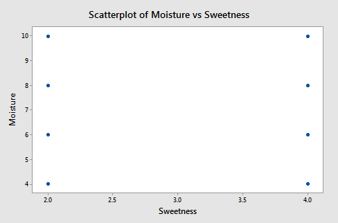
Notice that the points are on a rectangular grid so the correlation between the two variables is 0. (Please Note: we are not able to see that actually there are 2 observations at each location of the grid!)
The following figure shows how the two x-variables affect the pastry rating.
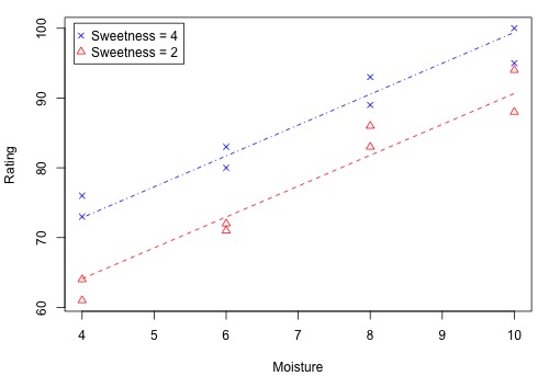
There is a linear relationship between rating and moisture and there is also a sweetness difference. The Minitab results given in the following output are for three different regressions - separate simple regressions for each x-variable and a multiple regression that incorporates both x-variables.
Regression Analysis: Rating versus Moisture
Analysis of Variance
| Source | DF | Adj SS | Adj MS | F-Value | P-value |
|---|---|---|---|---|---|
| Regression | 1 | 1566.45 | 1566.45 | 54.75 | 0.000 |
| Moisture | 1 | 166.45 | 1566.45 | 54.75 | 0.000 |
| Error | 14 | 400.55 | 28.61 | ||
| Lack-of-Fit | 2 | 15.05 | 7.52 | 0.23 | 0.795 |
| Pure Error | 12 | 385.50 | 32.13 | ||
| Total | 15 | 1967.00 |
Model Summary
| S | R-sq | R-sq(adj) | R-sq(pred) |
|---|---|---|---|
| 5.34890 | 79.64% | 78.18% | 72.71% |
Coefficients
| Term | Coef | SE Coef | T-Value | P-Value | VIF |
|---|---|---|---|---|---|
| Constant | 5077 | 4.39 | 11.55 | 0.000 | |
| Moisture | 4.425 | 0.598 | 7.40 | 0.000 | 1.00 |
Regression Equation
Rating = 50.77 + 4.425 Moisture
Regression Analysis: Rating versus Sweetness
Analysis of Variance
| Source | DF | Adj SS | Adj MS | F-Value | P-value |
|---|---|---|---|---|---|
| Regression | 1 | 306.3 | 306.3 | 2.58 | 0.130 |
| Sweetness | 1 | 306.3 | 306.3 | 2.58 | 0.130 |
| Error | 14 | 1660.8 | 118.6 | ||
| Total | 15 | 1967.0 |
Model Summary
| S | R-sq | R-sq(adj) | R-sq(pred) |
|---|---|---|---|
| 10.8915 | 15.57% | 9.54% | 0.00% |
Coefficients
| Term | Coef | SE Coef | T-Value | P-Value | VIF |
|---|---|---|---|---|---|
| Constant | 68.63 | 8.61 | 7.97 | 0.000 | |
| Sweetness | 4.38 | 2.72 | 1.61 | 0.130 | 1.00 |
Regression Equation
Rating = 68.63 + 4.38 Sweetness
Regression Analysis: Rating versus Moisture, Sweetness
Analysis of Variance
| Source | DF | Adj SS | Adj MS | F-Value | P-value |
|---|---|---|---|---|---|
| Regression | 2 | 1872.70 | 936.35 | 129.08 | 0.000 |
| Moisture | 1 | 1566.45 | 1566.45 | 215.95 | 0.000 |
| Sweetness | 1 | 306.25 | 306.25 | 42.22 | 0.000 |
| Error | 13 | 94.30 | 7.25 | ||
| Lack-of-Fit | 5 | 37.30 | 7.46 | 1.05 | 0.453 |
| 857.00 | 7.13 | ||||
| Total | 15 | 1967.00 |
Model Summary
| S | R-sq | R-sq(adj) | R-sq(pred) |
|---|---|---|---|
| 2.69330 | 95.21% | 94.47% | 92.46% |
Coefficients
| Term | Coef | SE Coef | T-Value | P-Value | VIF |
|---|---|---|---|---|---|
| Constant | 37.65 | 3.00 | 12.57 | 0.000 | |
| Moisture | 4.425 | 0.301 | 14.70 | 0.000 | 1.00 |
| Sweetness | 4.375 | 0.673 | 6.50 | 0.000 | 1.00 |
Regression Equation
Rating = 37.65 + 4.425 Moisture + 4.375 Sweetness
There are three important features to notice in the results:
-
The sample coefficient that multiplies Moisture is 4.425 in both the simple and the multiple regression. The sample coefficient that multiplies Sweetness is 4.375 in both the simple and the multiple regression. This result does not generally occur; the only reason that it does, in this case, is that Moisture and Sweetness are not correlated, so the estimated slopes are independent of each other. For most observational studies, predictors are typically correlated and estimated slopes in a multiple linear regression model do not match the corresponding slope estimates in simple linear regression models.
-
The \(R^{2}\) for the multiple regression, 95.21%, is the sum of the \(R^{2}\) values for the simple regressions (79.64% and 15.57%). Again, this will only happen when we have uncorrelated x-variables.
-
The variable Sweetness is not statistically significant in the simple regression (p = 0.130), but it is in the multiple regression. This is a benefit of doing a multiple regression. By putting both variables into the equation, we have greatly reduced the standard deviation of the residuals (notice the S values). This in turn reduces the standard errors of the coefficients, leading to greater t-values and smaller p-values.
(Data source: Applied Regression Models, (4th edition), Kutner, Neter, and Nachtsheim).
Example 5-5: Female Stat Students
The data are from n = 214 females in statistics classes at the University of California at Davis (Stat Females dataset). The variables are y = student’s self-reported height, \(x_{1}\) = student’s guess at her mother’s height, and \(x_{2}\) = student’s guess at her father’s height. All heights are in inches. The scatterplots below are of each student’s height versus the mother’s height and the student’s height against the father’s height.
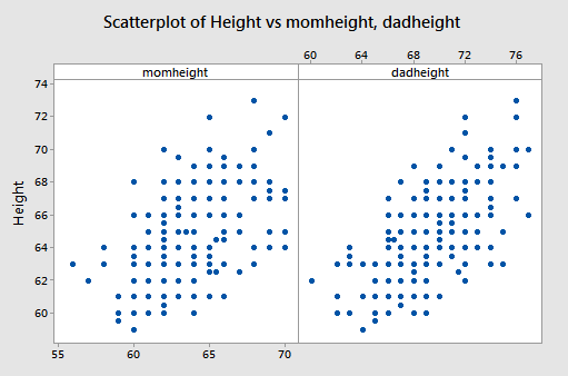
Both show a moderate positive association with a straight-line pattern and no notable outliers.
Interpretations
The first two lines of the Minitab output show that the sample multiple regression equations is predicted student height = 18.55 + 0.3035 × mother’s height + 0.3879 × father’s height:
Regression Analysis: Height versus momheight, dadheight
Analysis of Variance
| Source | DF | Adj SS | Adj MS | F-Value | P-value |
|---|---|---|---|---|---|
| Regression | 2 | 666.1 | 333.074 | 80.73 | 0.000 |
| momheight | 1 | 128.1 | 128.117 | 31.05 | 0.000 |
| dadheight | 1 | 278.5 | 278.488 | 67.50 | 0.000 |
| Error | 211 | 870.5 | 4.126 | ||
| Lack-of-Fit | 101 | 446.3 | 4.419 | 1.15 | 0.242 |
| Pure Error | 110 | 424.2 | 3.857 | ||
| Total | 213 | 1536.6 |
Model Summary
| S | R-sq | R-sq(adj) | R-sq(pred) |
|---|---|---|---|
| 2.03115 | 43.35% | 42.81% | 41.58% |
Coefficients
| Term | Coef | SE Coef | T-Value | P-Value | VIF |
|---|---|---|---|---|---|
| Constant | 18.55 | 3.69 | 5.02 | 0.000 | |
| momheight | 0.3035 | 0.0545 | 5.57 | 0.000 | 1.19 |
| dadheight | 0.3879 | 0.0472 | 8.22 | 0.000 | 1.19 |
Regression Equation
Rating = 18.55 + 0.3035 momheight + 0.3879 dadheight
To use this equation for prediction, we substitute specified values for the two parents’ heights.
We can interpret the “slopes” in the same way that we do for a simple linear regression model but we have to add the constraint that values of other variables remain constant. For example:
– When the father’s height is held constant, the average student height increases by 0.3035 inches for each one-inch increase in the mother’s height.
– When the mother’s height is held constant, the average student height increases by 0.3879 inches for each one-inch increase in the father’s height.
- The p-values given for the two x-variables tell us that student height is significantly related to each.
- The value of \(R^{2}\) = 43.35% means that the model (the two x-variables) explains 43.35% of the observed variation in student heights.
- The value S = 2.03115 is the estimated standard deviation of the regression errors. Roughly, it is the average absolute size of a residual.
Residual Plots
Just as in simple regression, we can use a plot of residuals versus fits to evaluate the validity of assumptions. The residual plot for these data is shown in the following figure:
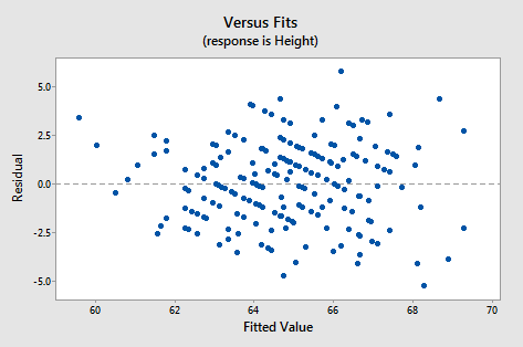
It looks about as it should - a random horizontal band of points. Other residual analyses can be done exactly as we did for simple regression. For instance, we might wish to examine a normal probability plot of the residuals. Additional plots to consider are plots of residuals versus each x-variable separately. This might help us identify sources of curvature or non-constant variance.
Example 5-6: Hospital Data
Data from n = 113 hospitals in the United States are used to assess factors related to the likelihood that a hospital patient acquires an infection while hospitalized. The variables here are y = infection risk, \(x_{1}\) = average length of patient stay, \(x_{2}\) = average patient age, \(x_{3}\) = measure of how many x-rays are given in the hospital (Hospital Infection dataset). The Minitab output is as follows:
Coefficients
| Term | Coef | SE Coef | T-Value | P-Value | VIF |
|---|---|---|---|---|---|
| Constant | 1.00 | 1.31 | 0.76 | 0.448 | |
| Stay | 0.3082 | 0.0594 | 5.19 | 0.000 | 1.23 |
| Age | -0.0230 | 0.0235 | -0.98 | 0.330 | 1.05 |
| Xray | 0.01966 | 0.00576 | 3.41 | 0.001 | 1.18 |
Regression Equation
InfctRsk = 1.00 + 0.3082 Stay - 0.0230 Age + 0.01966 Xray
Interpretations for this example include:
- The p-value for testing the coefficient that multiplies Age is 0.330. Thus we cannot reject the null hypothesis \(H_0 \colon \beta_{2}\) = 0. The variable Age is not a useful predictor within this model that includes Stay and Xrays.
- For the variables Stay and X-rays, the p-values for testing their coefficients are at a statistically significant level so both are useful predictors of infection risk (within the context of this model!).
- We usually don’t worry about the p-value for Constant. It has to do with the “intercept” of the model and seldom has any practical meaning. It also doesn’t give information about how changing an x-variable might change y-values.
(Data source: Applied Regression Models, (4th edition), Kutner, Neter, and Nachtsheim).
Example 5-7: Physiological Measurements Data
For a sample of n = 20 individuals, we have measurements of y = body fat, \(x_{1}\) = triceps skinfold thickness, \(x_{2}\) = thigh circumference, and \(x_{3}\) = midarm circumference (Body Fat dataset). Minitab results for the sample coefficients, MSE (highlighted), and \(\left(X^{T} X \right)^{−1}\) are given below:
Regression Analysis: Bodyfat versus Triceps, Thigh, Midarm
Analysis of Variance
| Source | DF | Adj SS | Adj MS | F-Value | P-Value |
|---|---|---|---|---|---|
| Regression | 3 | 396.985 | 132.328 | 21.52 | 0.000 |
| Triceps | 1 | 12.705 | 12.705 | 2.07 | 0.170 |
| Thigh | 1 | 7.529 | 7.529 | 1.22 | 0.285 |
| Midarm | 1 | 11.546 | 11.546 | 1.88 | 0.190 |
| Error | 16 | 98.405 | 6.150 | ||
| Total | 19 | 495.390 |
Model Summary
| S | R-sq | R-sq(adj) | R-sq(pred) |
|---|---|---|---|
| 2.47998 | 80.14% | 76.41% | 67.55% |
Coefficients
| Predictor | Coef | SE Coef | T-Value | P-Value | VIF |
|---|---|---|---|---|---|
| Constant | 117.1 | 99.8 | 1.17 | 0.258 | |
| Triceps | 4.33 | 3.02 | 1.44 | 0.170 | 708.84 |
| Thigh | -2.86 | 2.58 | -1.11 | 0.285 | 564.34 |
| Midarm | -2.19 | 1.60 | -1.37 | 0.190 | 104.61 |
Regression Equation
Bodyfat 117.1 + 4.33 Triceps - 2.86 Thigh - 2.19 Midarm
\(\left(X^{T} X \right)^{−1}\) - (calculated manually, see note below)
| Body Fat Calculations | |||
|---|---|---|---|
| 1618.87 | 48.8103 | -41.8487 | -25.7988 |
| 48.81 | 1.4785 | -1.2648 | -0.7785 |
| -41.85 | -1.2648 | 1.0840 | 0.6658 |
| -25.80 | -0.7785 | 0.6658 | 0.4139 |
The variance-covariance matrix of the sample coefficients is found by multiplying each element in \(\left(X^{T} X \right)^{−1}\) by MSE. Common notation for the resulting matrix is either \(s^{2}\)(b) or \(se^{2}\)(b). Thus, the standard errors of the coefficients given in the Minitab output can be calculated as follows:
- Var(\(b_{0}\)) = (6.15031)(1618.87) = 9956.55, so se(\(b_{0}\)) = \(\sqrt{9956.55}\) = 99.782.
- Var(\(b_{1}\)) = (6.15031)(1.4785) = 9.0932, so se(\(b_{1}\)) = \(\sqrt{9.0932}\) = 3.016.
- Var(\(b_{2}\)) = (6.15031)(1.0840) = 6.6669, so se(\(b_{2}\)) = \(\sqrt{6.6669}\) = 2.582.
- Var(\(b_{3}\)) = (6.15031)(0.4139) = 2.54561, so se(\(b_{3}\)) = \(\sqrt{2.54561}\) = 1.595.
As an example of covariance and correlation between two coefficients, we consider \(b_{1 }\)and \(b_{2}\).
- Cov(\(b_{1}\), \(b_{2}\)) = (6.15031)(−1.2648) = −7.7789. The value -1.2648 is in the second row and third column of \(\left(X^{T} X \right)^{−1}\). (Keep in mind that the first row and first column give information about \(b_0\), so the second row has information about \(b_{1}\), and so on.)
- Corr(\(b_{1}\), \(b_{2}\)) = covariance divided by product of standard errors = −7.7789 / (3.016 × 2.582) = −0.999.
The extremely high correlation between these two sample coefficient estimates results from a high correlation between the Triceps and Thigh variables. The consequence is that it is difficult to separate the individual effects of these two variables.
If all x-variables are uncorrelated with each other, then all covariances between pairs of sample coefficients that multiply x-variables will equal 0. This means that the estimate of one beta is not affected by the presence of the other x-variables. Many experiments are designed to achieve this property. With observational data, however, we’ll most likely not have this happen.
(Data source: Applied Regression Models, (4th edition), Kutner, Neter, and Nachtsheim).
Software Help 5
Software Help 5
Help
The next two pages cover the Minitab and R commands for the procedures in this lesson.
Below is a zip file that contains all the data sets used in this lesson:
- babybirds.txt
- bodyfat.txt
- hospital_infct.txt
- fev_dat.txt
- iqsize.txt
- pastry.txt
- soapsuds.txt
- stat_females.txt
Minitab Help 5: Multiple Linear Regression
Minitab Help 5: Multiple Linear RegressionMinitab®
IQ and physical characteristics
- Create a simple matrix of scatter plots.
- Perform a linear regression analysis of PIQ on Brain, Height, and Weight.
- Click "Options" in the regression dialog to choose between Sequential (Type I) sums of squares and Adjusted (Type III) sums of squares in the Anova table.
Underground air quality
- Create a simple matrix of scatter plots.
- Select Graph > 3D Scatterplot (Simple) to create a 3D scatterplot of the data.
- Perform a linear regression analysis of Vent on O2 and CO2.
- Click "Options" in the regression dialog to choose between Sequential (Type I) sums of squares and Adjusted (Type III) sums of squares in the Anova table.
Soapsuds example (using matrices)
- Perform a linear regression analysis of suds on soap.
- Click "Storage" in the regression dialog and check "Design matrix" to store the design matrix, X.
- To create \(X^T\): Select Calc > Matrices > Transpose, select "XMAT" to go into the "Transpose from" box, and type "M2" in the "Store result in" box.
- To calculate \(X^{T} X\): Select Calc > Matrices > Arithmetic, click "Multiply," select "M2" to go in the left-hand box, select "XMAT" to go in the right-hand box, and type "M3" in the "Store result in" box. Display the result by selecting Data > Display Data.
- To calculate \(X^{T} Y\): Select Calc > Matrices > Arithmetic, click "Multiply," select "M2" to go in the left-hand box, select "suds" to go in the right-hand box, and type "M4" in the "Store result in" box. Display the result by selecting Data > Display Data.
- To calculate \(\left(X^{T}X\right)^{-1} \colon \) Select Calc > Matrices > Invert, select "M3" to go in the "Invert from" box, and type "M5" in the "Store result in" box. Display the result by selecting Data > Display Data.
- To calculate b = \(\left(X^{T}X\right)^{-1} X^{T} Y \colon \) Select Calc > Matrices > Arithmetic, click "Multiply," select "M5" to go in the left-hand box, select "M4" to go in the right-hand box, and type "M6" in the "Store result in" box. Display the result by selecting Data > Display Data.
Pastry sweetness
- Obtain a sample correlation
- Create a basic scatterplot.
- Perform a linear regression analysis of Rating on Moisture and Sweetness.
- Click "Storage" in the regression dialog and check "Fits" to store the fitted (predicted) values.
- To create a scatterplot of the data with points marked by Sweetness and two lines representing the fitted regression equation for each group:
- Select Calc > Calculator, type "FITS_2" in the "Store result in variable" box, and type "IF('Sweetness'=2,'FITS')" in the "Expression" box. Repeat for FITS_4 (Sweetness=4).
- Create a basic scatter plot but select "With Groups" instead of "Simple." Select Rating as the "Y variable," Moisture as the "X variable," and Sweetness as the "Categorical variable for grouping."
- Select Editor > Add > Calculated Line and select "FITS_2" to go into the "Y column" and "Moisture" to go into the "X column." Repeat for FITS_4 (Sweetness=4).
- Perform a linear regression analysis of Rating on Moisture.
- Perform a linear regression analysis of Rating on Sweetness.
Female stat students
- Create a simple matrix of scatter plots.
- Perform a linear regression analysis of Height on momheight and dadheight.
- Create residual plots and select "Residuals versus fits" (with regular residuals).
Hospital infections
- Perform a linear regression analysis of InfctRsk on Stay, Age, and Xray.
Physiological measurements (using matrices)
- Perform a linear regression analysis of BodyFat on Triceps, Thigh, and Midarm.
- Click "Storage" in the regression dialog and check "Design matrix" to store the design matrix, X.
- To create \(X^T\): Select Calc > Matrices > Transpose, select "XMAT" to go into the "Transpose from" box, and type "M2" in the "Store result in" box.
- To calculate \(X^{T} X\): Select Calc > Matrices > Arithmetic, click "Multiply," select "M2" to go in the left-hand box, select "XMAT" to go in the right-hand box, and type "M3" in the "Store result in" box. Display the result by selecting Data > Display Data.
- To calculate \(\left(X^{T}X\right)^{-1} \colon \) Select Calc > Matrices > Invert, select "M3" to go in the "Invert from" box, and type "M4" in the "Store result in" box. Display the result by selecting Data > Display Data.
Peruvian blood pressure
- Use Calc > Calculator to calculate FracLife variable.
- Perform a linear regression analysis of Systol on nine predictors.
- Perform a linear regression analysis of Systol on four predictors.
- Find an F-based P-value.
Measurements of college students
- Perform a linear regression analysis of Height on LeftArm, LeftFoot, HeadCirc, and nose.
- Create residual plots and select "Residuals versus fits" (with regular residuals).
- Perform a linear regression analysis of Height on LeftArm and LeftFoot.
- Find an F-based P-value.
- Perform a linear regression analysis of Height on LeftFoot.
R Help 5: Multiple Linear Regression
R Help 5: Multiple Linear RegressionR Help
IQ and physical characteristics
- Load the iqsize data.
- Display a scatterplot matrix of the data.
- Fit a multiple linear regression model of PIQ on Brain, Height, and Weight.
- Display model results.
- Use the
anovafunction to display the ANOVA table with sequential (type I) sums of squares. - Use the
Anovafunction from thecarpackage to display the ANOVA table with adjusted (type III) sums of squares.
iqsize <- read.table("~/path-to-folder/iqsize.txt", header=T)
attach(iqsize)

pairs(cbind(PIQ, Brain, Height, Weight))

model <- lm(PIQ ~ Brain + Height + Weight)
summary(model)
# Coefficients:
#               Estimate Std. Error t value Pr(>|t|)
# (Intercept)  1.114e+02  6.297e+01   1.768 0.085979 .
# Brain        2.060e+00  5.634e-01   3.657 0.000856 ***
# Height      -2.732e+00  1.229e+00  -2.222 0.033034 *
# Weight       5.599e-04  1.971e-01   0.003 0.997750
# ---
# Signif. codes:  0 ‘***’ 0.001 ‘**’ 0.01 ‘*’ 0.05 ‘.’ 0.1 ‘ ’ 1
#
# Residual standard error: 19.79 on 34 degrees of freedom
# Multiple R-squared:  0.2949,  Adjusted R-squared:  0.2327
# F-statistic: 4.741 on 3 and 34 DF,  p-value: 0.007215

anova(model) # Sequential (type I) SS
# Analysis of Variance Table
# Response: PIQ
#           Df  Sum Sq Mean Sq F value  Pr(>F)
# Brain      1  2697.1 2697.09  6.8835 0.01293 *
# Height     1  2875.6 2875.65  7.3392 0.01049 *
# Weight     1     0.0    0.00  0.0000 0.99775
# Residuals 34 13321.8  391.82
# ---
# Signif. codes:  0 ‘***’ 0.001 ‘**’ 0.01 ‘*’ 0.05 ‘.’ 0.1 ‘ ’ 1

library(car)
Anova(model, type="III") # Adjusted (type III) SS
# Anova Table (Type III tests)
# Response: PIQ
#              Sum Sq Df F value    Pr(>F)
# (Intercept)  1225.2  1  3.1270 0.0859785 .
# Brain        5239.2  1 13.3716 0.0008556 ***
# Height       1934.7  1  4.9378 0.0330338 *
# Weight          0.0  1  0.0000 0.9977495
# Residuals   13321.8 34
# ---
# Signif. codes:  0 ‘***’ 0.001 ‘**’ 0.01 ‘*’ 0.05 ‘.’ 0.1 ‘ ’ 1

detach(iqsize)
Underground air quality
- Load the babybirds data.
- Display a scatterplot matrix of the data.
- Use the
scatter3dfunction from thecarpackage to create a 3D scatterplot of the data. - Fit a multiple linear regression model of Vent on O2 and CO2.
- Display model results.
- Use the
Anovafunction from thecarpackage todisplay the ANOVA table with adjusted (type III) sums of squares.
babybirds <- read.table("~/path-to-folder/babybirds.txt", header=T)
attach(babybirds)

pairs(cbind(Vent, O2, CO2))

library(car)
scatter3d(Vent ~ O2 + CO2)
scatter3d(Vent ~ O2 + CO2, revolutions=3, speed=0.5, grid=F)

model <- lm(Vent ~ O2 + CO2)
summary(model)
# Coefficients:
#             Estimate Std. Error t value Pr(>|t|)
# (Intercept)   85.901    106.006   0.810    0.419
# O2            -5.330      6.425  -0.830    0.408
# CO2           31.103      4.789   6.495  2.1e-09 ***
# ---
# Signif. codes:  0 ‘***’ 0.001 ‘**’ 0.01 ‘*’ 0.05 ‘.’ 0.1 ‘ ’ 1
#
# Residual standard error: 157.4 on 117 degrees of freedom
# Multiple R-squared:  0.2682,  Adjusted R-squared:  0.2557
# F-statistic: 21.44 on 2 and 117 DF,  p-value: 1.169e-08

Anova(model, type="III") # Adjusted (type III) SS
# Anova Table (Type III tests)
# Response: Vent
#              Sum Sq  Df F value    Pr(>F)
# (Intercept)   16262   1  0.6566    0.4194
# O2            17045   1  0.6883    0.4084
# CO2         1044773   1 42.1866 2.104e-09 ***
# Residuals   2897566 117
# ---
# Signif. codes:  0 ‘***’ 0.001 ‘**’ 0.01 ‘*’ 0.05 ‘.’ 0.1 ‘ ’ 1

detach(babybirds)
Soapsuds example (using matrices)
- Load the soapsuds data.
- Fit a simple linear regression model of suds on soap and store the model matrix, X.
- Display model results.
- Calculate \(X^{T}X , X^{T}Y , (X^{T} X)^{-1}\) , and \(b = (X^{T}X)^{-1} X^{T}Y\) .
- Fit a multiple linear regression model with linearly dependent predictors.
soapsuds <- read.table("~/path-to-folder/soapsuds.txt", header=T)
attach(soapsuds)

model <- lm(suds ~ soap, x=T)
summary(model)
# Coefficients:
#             Estimate Std. Error t value Pr(>|t|)
# (Intercept)  -2.6786     4.2220  -0.634    0.554
# soap          9.5000     0.7553  12.579 5.64e-05 ***

X <- model$x
t(X) %*% X
#             (Intercept)   soap
# (Intercept)         7.0  38.50
# soap               38.5 218.75

t(X) %*% suds
#             [,1]
# (Intercept)  347
# soap        1975

solve(t(X) %*% X)
#             (Intercept)       soap
# (Intercept)   4.4642857 -0.7857143
# soap         -0.7857143  0.1428571

solve(t(X) %*% X) %*% (t(X) %*% suds)
#                  [,1]
# (Intercept) -2.678571
# soap         9.500000

soap2 <- 2*soap
model <- lm(suds ~ soap + soap2)
summary(model)
# Coefficients: (1 not defined because of singularities)
#             Estimate Std. Error t value Pr(>|t|)
# (Intercept)  -2.6786     4.2220  -0.634    0.554
# soap          9.5000     0.7553  12.579 5.64e-05 ***
# soap2             NA         NA      NA       NA

detach(soapsuds)
Pastry sweetness
- Load the pastry data.
- Calculate the correlation between the predictors and create a scatterplot.
- Fit a multiple linear regression model of Rating on Moisture and Sweetness and display the model results.
- Create a scatterplot of the data with points marked by Sweetness and two lines representing the fitted regression equation for each sweetness level.
- Fit a simple linear regression model of Rating on Moisture and display the model results.
- Fit a simple linear regression model of Rating on Sweetness and display the model results.
pastry <- read.table("~/path-to-folder/pastry.txt", header=T)
attach(pastry)

cor(Sweetness, Moisture) # 0
plot(Sweetness, Moisture)

model.12 <- lm(Rating ~ Moisture + Sweetness)
summary(model.12)
#             Estimate Std. Error t value Pr(>|t|)
# (Intercept)  37.6500     2.9961  12.566 1.20e-08 ***
# Moisture      4.4250     0.3011  14.695 1.78e-09 ***
# Sweetness     4.3750     0.6733   6.498 2.01e-05 ***
# ---
# Signif. codes:  0 ‘***’ 0.001 ‘**’ 0.01 ‘*’ 0.05 ‘.’ 0.1 ‘ ’ 1
#
# Residual standard error: 2.693 on 13 degrees of freedom
# Multiple R-squared:  0.9521,  Adjusted R-squared:  0.9447
# F-statistic: 129.1 on 2 and 13 DF,  p-value: 2.658e-09

plot(Moisture, Rating, type="n")
for (i in 1:16) points(Moisture[i], Rating[i], pch=Sweetness[i], col=Sweetness[i])
for (i in c(2,4)) lines(Moisture[Sweetness==i], fitted(model.12)[Sweetness==i],
                        lty=i, col=i)
legend("topleft", legend=c("Sweetness = 4",
                           "Sweetness = 2"),
       col=c(4,2), pch=c(4,2), inset=0.02)

model.1 <- lm(Rating ~ Moisture)
summary(model.1)
#             Estimate Std. Error t value Pr(>|t|)
# (Intercept)   50.775      4.395  11.554 1.52e-08 ***
# Moisture       4.425      0.598   7.399 3.36e-06 ***
# ---
# Signif. codes:  0 ‘***’ 0.001 ‘**’ 0.01 ‘*’ 0.05 ‘.’ 0.1 ‘ ’ 1
#
# Residual standard error: 5.349 on 14 degrees of freedom
# Multiple R-squared:  0.7964,  Adjusted R-squared:  0.7818
# F-statistic: 54.75 on 1 and 14 DF,  p-value: 3.356e-06

model.2 <- lm(Rating ~ Sweetness)
summary(model.2)
#             Estimate Std. Error t value Pr(>|t|)
# (Intercept)   68.625      8.610   7.970 1.43e-06 ***
# Sweetness      4.375      2.723   1.607     0.13
# ---
# Signif. codes:  0 ‘***’ 0.001 ‘**’ 0.01 ‘*’ 0.05 ‘.’ 0.1 ‘ ’ 1
#
# Residual standard error: 10.89 on 14 degrees of freedom
# Multiple R-squared:  0.1557,  Adjusted R-squared:  0.09539
# F-statistic: 2.582 on 1 and 14 DF,  p-value: 0.1304

detach(pastry)
Female stat students
- Load the statfemales data.
- Display a scatterplot matrix of the data.
- Fit a multiple linear regression model of Height on momheight and dadheight and display the model results.
- Create a residual plot.
statfemales <- read.table("~/path-to-folder/stat_females.txt", header=T)
attach(statfemales)

pairs(cbind(Height, momheight, dadheight))

model <- lm(Height ~ momheight + dadheight)
summary(model)
#             Estimate Std. Error t value Pr(>|t|)
# (Intercept) 18.54725    3.69278   5.023 1.08e-06 ***
# momheight    0.30351    0.05446   5.573 7.61e-08 ***
# dadheight    0.38786    0.04721   8.216 2.10e-14 ***
# ---
# Signif. codes:  0 ‘***’ 0.001 ‘**’ 0.01 ‘*’ 0.05 ‘.’ 0.1 ‘ ’ 1
#
# Residual standard error: 2.031 on 211 degrees of freedom
# Multiple R-squared:  0.4335,  Adjusted R-squared:  0.4281
# F-statistic: 80.73 on 2 and 211 DF,  p-value: < 2.2e-16

plot(fitted(model), residuals(model),
     panel.last = abline(h=0, lty=2))

detach(statfemales)
Hospital infections
- Load the infectionrisk data.
- Fit a multiple linear regression model of InfctRsk on Stay, Age, and Xray and display the model results.
infectionrisk <- read.table("~/path-to-folder/infectionrisk.txt", header=T)
attach(infectionrisk)

model <- lm(InfctRsk ~ Stay + Age + Xray)
summary(model)
#              Estimate Std. Error t value Pr(>|t|)
# (Intercept)  1.001162   1.314724   0.761 0.448003
# Stay         0.308181   0.059396   5.189 9.88e-07 ***
# Age         -0.023005   0.023516  -0.978 0.330098
# Xray         0.019661   0.005759   3.414 0.000899 ***
# ---
# Signif. codes:  0 ‘***’ 0.001 ‘**’ 0.01 ‘*’ 0.05 ‘.’ 0.1 ‘ ’ 1
#
# Residual standard error: 1.085 on 109 degrees of freedom
# Multiple R-squared:  0.363,  Adjusted R-squared:  0.3455
# F-statistic:  20.7 on 3 and 109 DF,  p-value: 1.087e-10

detach(infectionrisk)
Physiological measurements (using matrices)
- Load the bodyfat data.
- Fit a multiple linear regression model of BodyFat on Triceps, Thigh, and Midarm and store the model matrix, X.
- Display model results.
- Calculate MSE and \((X^{T} X)^{-1}\) and multiply them to find the variance-covariance matrix of the regression parameters.
- Use the variance-covariance matrix of the regression parameters to derive:
- the regression parameter standard errors.
- covariances and correlations between regression parameter estimates.
bodyfat <- read.table("~/path-to-folder/bodyfat.txt", header=T)
attach(bodyfat)

model <- lm(Bodyfat ~ Triceps + Thigh + Midarm, x=T)
summary(model)
#             Estimate Std. Error t value Pr(>|t|)
# (Intercept)  117.085     99.782   1.173    0.258
# Triceps        4.334      3.016   1.437    0.170
# Thigh         -2.857      2.582  -1.106    0.285
# Midarm        -2.186      1.595  -1.370    0.190
#
# Residual standard error: 2.48 on 16 degrees of freedom
# Multiple R-squared:  0.8014,  Adjusted R-squared:  0.7641
# F-statistic: 21.52 on 3 and 16 DF,  p-value: 7.343e-06

anova(model)
#           Df Sum Sq Mean Sq F value    Pr(>F)
# Triceps    1 352.27  352.27 57.2768 1.131e-06 ***
# Thigh      1  33.17   33.17  5.3931   0.03373 *
# Midarm     1  11.55   11.55  1.8773   0.18956
# Residuals 16  98.40    6.15
# ---
# Signif. codes:  0 ‘***’ 0.001 ‘**’ 0.01 ‘*’ 0.05 ‘.’ 0.1 ‘ ’ 1

MSE <- sum(residuals(model)^2)/model$df.residual # 6.150306
X <- model$x
XTXinv <- solve(t(X) %*% X)
#             (Intercept)    Triceps       Thigh      Midarm
# (Intercept)  1618.86721 48.8102522 -41.8487041 -25.7987855
# Triceps        48.81025  1.4785133  -1.2648388  -0.7785022
# Thigh         -41.84870 -1.2648388   1.0839791   0.6657581
# Midarm        -25.79879 -0.7785022   0.6657581   0.4139009

sqrt(MSE*diag(XTXinv)) # standard errors of the regression parameters
# (Intercept)     Triceps       Thigh      Midarm
#   99.782403    3.015511    2.582015    1.595499

MSE*XTXinv[2,3] # cov(b1, b2) = -7.779145
XTXinv[2,3]/sqrt(XTXinv[2,2]*XTXinv[3,3]) # cor(b1, b2) = -0.9991072

detach(bodyfat)
Peruvian blood pressure
- Load the peru data.
- Calculate FracLife variable.
- Fit full multiple linear regression model of Systol on nine predictors.
- Fit reduced multiple linear regression model of Systol on four predictors.
- Calculate SSE for the full and reduced models.
- Calculate the general linear F statistic by hand and find the p-value.
- Use the
anovafunction with full and reduced models to display F-statistic and p-value directly.
peru <- read.table("~/path-to-folder/peru.txt", header=T)
attach(peru)

FracLife <- Years/Age

model.1 <- lm(Systol ~ Age + Years + FracLife + Weight + Height + Chin +
              Forearm + Calf + Pulse)
summary(model.1)
#               Estimate Std. Error t value Pr(>|t|)
# (Intercept)  146.81907   48.97096   2.998 0.005526 **
# Age           -1.12144    0.32741  -3.425 0.001855 **
# Years          2.45538    0.81458   3.014 0.005306 **
# FracLife    -115.29395   30.16900  -3.822 0.000648 ***
# Weight         1.41393    0.43097   3.281 0.002697 **
# Height        -0.03464    0.03686  -0.940 0.355194
# Chin          -0.94369    0.74097  -1.274 0.212923
# Forearm       -1.17085    1.19329  -0.981 0.334612
# Calf          -0.15867    0.53716  -0.295 0.769810
# Pulse          0.11455    0.17043   0.672 0.506818

anova(model.1)
#           Df  Sum Sq Mean Sq F value    Pr(>F)
# Age        1    0.22    0.22  0.0030  0.956852
# Years      1   82.55   82.55  1.1019  0.302514
# FracLife   1 3112.41 3112.41 41.5449 4.728e-07 ***
# Weight     1  706.54  706.54  9.4311  0.004603 **
# Height     1    1.68    1.68  0.0224  0.882117
# Chin       1  297.68  297.68  3.9735  0.055704 .
# Forearm    1  113.91  113.91  1.5205  0.227440
# Calf       1   10.01   10.01  0.1336  0.717420
# Pulse      1   33.84   33.84  0.4518  0.506818
# Residuals 29 2172.58   74.92

model.2 <- lm(Systol ~ Age + Years + FracLife + Weight)
summary(model.2)
#              Estimate Std. Error t value Pr(>|t|)
# (Intercept)  116.8354    21.9797   5.316 6.69e-06 ***
# Age           -0.9507     0.3164  -3.004 0.004971 **
# Years          2.3393     0.7714   3.032 0.004621 **
# FracLife    -108.0728    28.3302  -3.815 0.000549 ***
# Weight         0.8324     0.2754   3.022 0.004742 **

anova(model.2)
#           Df  Sum Sq Mean Sq F value    Pr(>F)
# Age        1    0.22    0.22  0.0029  0.957480
# Years      1   82.55   82.55  1.0673  0.308840
# FracLife   1 3112.41 3112.41 40.2409 3.094e-07 ***
# Weight     1  706.54  706.54  9.1350  0.004742 **
# Residuals 34 2629.71   77.34

(2629.71-2172.58)/(34-29) / (2172.58/29) # F = 1.220371
pf(1.220371, 5, 29, lower.tail=F) # p-value = 0.3247213

anova(model.2, model.1)
#   Res.Df    RSS Df Sum of Sq      F Pr(>F)
# 1     34 2629.7
# 2     29 2172.6  5    457.12 1.2204 0.3247

detach(peru)
Measurements of college students
- Load the Physical data.
- Fit full multiple linear regression model of Height on LeftArm, LeftFoot, HeadCirc, and nose.
- Create a residual plot.
- Fit reduced multiple linear regression model of Height on LeftArm and LeftFoot.
- Calculate SSE for the full and reduced models.
- Calculate the general linear F statistic by hand and find the p-value.
- Use the
anovafunction with full and reduced models to display F-statistic and p-value directly. - Calculate partial R-squared for (LeftArm | LeftFoot).
physical <- read.table("~/path-to-folder/Physical.txt", header=T)
attach(physical)

model.1 <- lm(Height ~ LeftArm + LeftFoot + HeadCirc + nose)
summary(model.1)
#             Estimate Std. Error t value Pr(>|t|)
# (Intercept) 18.50265    7.83031   2.363   0.0221 *
# LeftArm      0.80205    0.17074   4.697 2.09e-05 ***
# LeftFoot     0.99730    0.16230   6.145 1.30e-07 ***
# HeadCirc     0.08052    0.14952   0.539   0.5926
# nose        -0.14740    0.49233  -0.299   0.7659

plot(fitted(model.1), residuals(model.1),
     panel.last = abline(h=0, lty=2))

anova(model.1)
#           Df Sum Sq Mean Sq  F value    Pr(>F)
# LeftArm    1 590.21  590.21 123.8106 3.917e-15 ***
# LeftFoot   1 224.35  224.35  47.0621 9.931e-09 ***
# HeadCirc   1   1.40    1.40   0.2940    0.5901
# nose       1   0.43    0.43   0.0896    0.7659
# Residuals 50 238.35    4.77

model.2 <- lm(Height ~ LeftArm + LeftFoot)
summary(model.2)
#             Estimate Std. Error t value Pr(>|t|)
# (Intercept)  21.8572     3.5840   6.098 1.35e-07 ***
# LeftArm       0.7958     0.1652   4.816 1.31e-05 ***
# LeftFoot      1.0229     0.1468   6.969 5.54e-09 ***

anova(model.2)
#           Df Sum Sq Mean Sq F value    Pr(>F)
# LeftArm    1 590.21  590.21 127.782 1.275e-15 ***
# LeftFoot   1 224.35  224.35  48.572 5.538e-09 ***
# Residuals 52 240.18    4.62

(240.18-238.35)/(52-50) / (238.35/50) # F = 0.1919446
pf(0.1919446, 2, 50, lower.tail=F) # p-value = 0.8259579

anova(model.2, model.1)
#   Res.Df    RSS Df Sum of Sq      F Pr(>F)
# 1     52 240.18
# 2     50 238.35  2    1.8289 0.1918 0.8261

model.3 <- lm(Height ~ LeftFoot)
anova(model.3)
#           Df Sum Sq Mean Sq F value    Pr(>F)
# LeftFoot   1 707.42  707.42  107.95 2.172e-14 ***
# Residuals 53 347.33    6.55

(347.33-240.18) / 347.33 # Partial R-squared (LeftArm | LeftFoot) = 0.3084962

detach(physical)