Example - Horseshoe Crabs and Satellites
 Please Note: This page is devoted entirely to working this example through using R, the previous page examined the same example using SAS.
 This problem refers to data from a study of nesting horseshoe crabs (J. Brockmann, Ethology 1996); see also Agresti (1996) Sec. 4.3 and Agresti (2002) Sec. 4.3. Each female horseshoe crab in the study had a male crab attached to her in her nest. The study investigated factors that affect whether the female crab had any other males, called satellites, residing near her. Explanatory variables that are thought to affect this included the female crab’s color (C), spine condition (S), weight (Wt), and carapace width (W). The response outcome for each female crab is her number of satellites (Sa). There are 173 females in this study. Datafile: crab.txt.
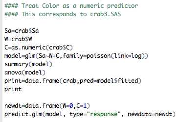
Let’s first see if the width of female's back can explain the number of satellites attached. We will start by fitting a Poisson regression model with only one predictor, width (W) via GLM( ) in Crab.R Program:
Below is the part of R code that corresponds to the SAS code on the previous page for fitting a Poisson regression model with only one predictor, carapace width (W).
#### Poisson Regression of Sa on W

model=glm(crab$Sa~1+crab$W,family=poisson(link=log))
Note that the specification of a Poisson distribution in R is “family=poisson” and “link=log”. You can also get the predicted count for each observation and the linear predictor values from R output by using specific statements such as:
#### to get the predicted count for each observation:
#### e.g. for the first observation E(y1)=3.810

print=data.frame(crab,pred=model$fitted)
print

#### note the linear predictor values
#### e.g., for the first observation, exp(1.3378)=3.810

model$linear.predictors
exp(model$linear.predictors)
In the output below, you should be able to identify the relevant parts:
- What do you learn from "summary(model)"? How is this different from when we fitted logistic regression models?
- Does the model fit well? What does the Value/DF tell you?
- Is width the significant predictor?
Here is the output:
The estimated model is: $log (\hat{\mu_i})$ = -3.30476 + 0.16405Wi
The ASE of estimated β = 0.164 is 0.01997 which is small, and the slope is statistically significant given its z-value of 8.216 and its low p-value.
Interpretation: Since estimate of β > 0, the wider the female crab, the greater expected number of male satellites on the multiplicative order as exp(0.1640) = 1.18. More specifically, for one unit of increase in the width, the number of Sa will increase and it will be multiplied by 1.18.
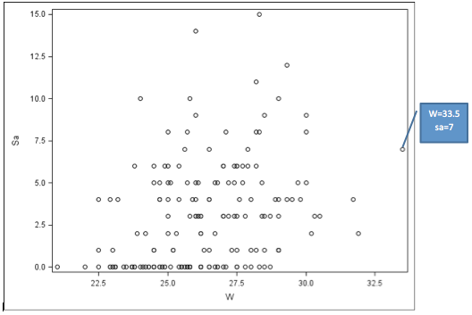
If we look at the scatter plot of W vs. Sa (see further below) we may suspect some outliers, e.g., observations #48, #101 and #165. For example, #165 has W = 33.5, and Sa = 7. But by studying the residuals, we see that this is not an influential observation, e.g., standardized deviance residual is -0.739 from running rstandard(model).
161 162 163 164 165 166 167 168 169 170
-0.16141380 -0.44808356 0.19325932 0.55048032 -0.73914681 -2.25624217 4.16609739 -1.81423271 -2.77425867 0.65241355
You can consider other types of residuals, influence measures (like we saw in linear regression), as well as residual plots. Notice that there are some other points that have large outliers, e.g., #101.
Here is a part of the output from running the other part of R code:
From the above output we can see the predicted counts ("fitted") and the values of the linear predictor that is the log of the expected counts. For example, for the first observation, pred = 3.810, linear.predictors = 1.3377, log(pred) = linear.predictors, that is log(3.810) = 1.3377, or exp(linear.predictors) = pred, that is exp(1.3377) = 3.810.
We can also see that although the predictor is significant the model does not fit well. Given the value of the residual deviance statistic of 567.88 with 171 df, the p-value is zero and the Value/DF=567.88/171=3.321 is much bigger than 1, so the model does not fit well. The lack of fit maybe due to missing data, covariates or overdispersion.

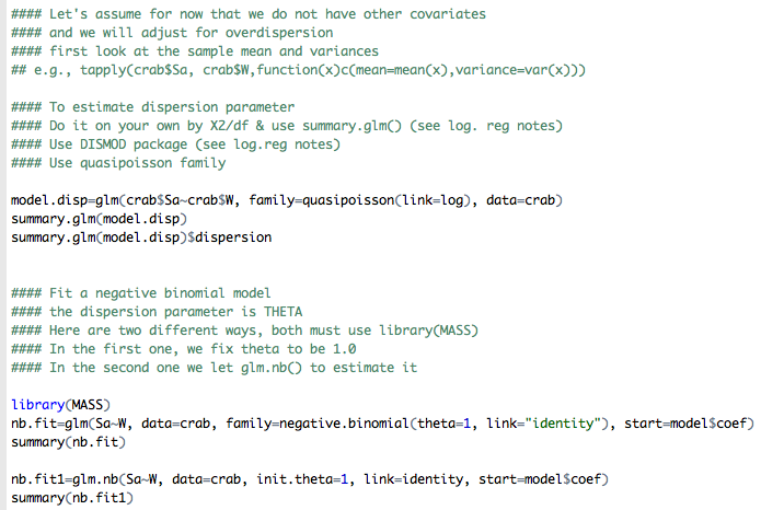
Let us assume for now that we do not have any other covariates, and try to adjust for overdispersion to see if we can improve the model fit.
Change the Model: Adjusting for Overdispersion
In the above model we detect a potential problem with overdispersion since the scale factor, e.g., Value/DF for the residual deviance/df, is much greater than 1.
What do you think overdispersion means for Poisson Regression? What does it tell you about the relationship between the mean and the variance of the Poisson distribution for the number of satellites? Recall that one of the reasons for overdispersion is heterogeneity where subjects within each covariate combination still differ greatly (i.e., even crabs with similar width will have different number of satellites). If that's the case, which assumption of the Poisson model that is Poisson regression model is violated?
Below is an example R code to estimate the dispersion parameter. Note that we specify “family=quasipossion” and only one covariate “crab$W” in the statement. We can also fit a negative binomial regression instead; for this see the crab.r code.
The output from the above R program:
With this model the random component does not have a Poisson distribution any more where the response has the same mean and variance. From the estimate given (e.g., Pearson X2 = 3.1822), the variance of random component (response, the number of satellites for each Width) is roughly three times the size of the mean.
The new standard errors (in comparison to the model where scale = 1), are larger, e.g., 0.0356 = 1.7839 × 0.02. Thus the Wald X2 statistics will be smaller, e.g., 21.22 = 67.21 / 3.1822. Note that sqrt(3.1822) = 1.7839.
What could be another reason for poor fit besides overdispersion? How about missing other explanatory variables? Can we improve the fit by adding other variables?
Change the Model: Include ‘color’ as a Qualitative Predictor
The following change is reflected in this part of R code to match the code in SAS on the previous page (this clearly does not need to be done).
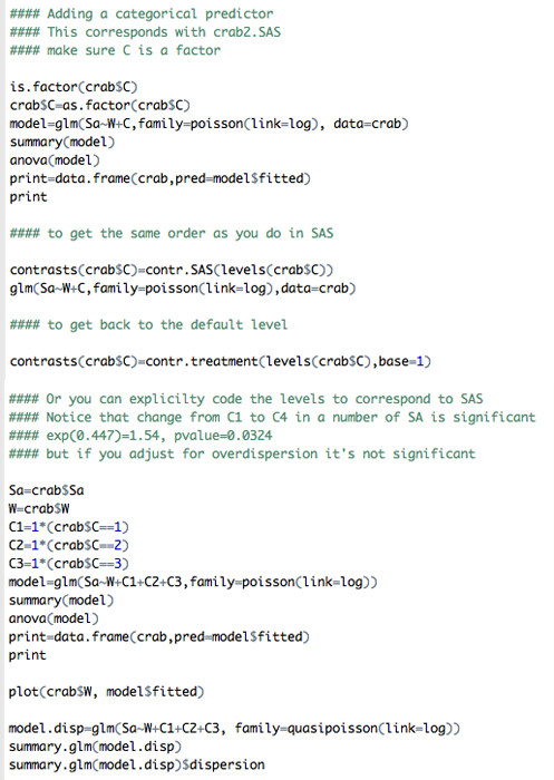
Let's compare the parts of this output with the model only having “W” as predictor. We are introducing "dummy variables" into the model to represent the color variable that has 4 levels with the level #4 as the reference level. We are also adjusting for overdispersion but by using deviance instead of X2 with option quasipoisson, although scale by pearson is preferred; we are doing this to demonstrate possible options in R and since the values are close, it doesn't matter which option we are using!
The estimated model is: $\log{\hat{\mu_i}}$= -3.0974 + 0.1493W + 0.4474(C="1") + 0.2477(C="2") + 0.0110(C="3").
There does not seem to be a difference in the number of satellites between any color class and the reference level 4 according to the t-value statistics for each row in the table above. Furthermore, if you run anova(model.disp), from output below we see that the color is barely overall statistically significant predictor after we take the width into consideration.
> anova(model.disp)
Analysis of Deviance Table
Model: quasipoisson, link: log
Response: Sa
Terms added sequentially (first to last)
Df Deviance Resid. Df Resid. Dev
NULL 172 632.79
W 1 64.913 171 567.88
C1 1 3.130 170 564.75
C2 1 5.400 169 559.35
C3 1 0.004 168 559.34
Does this model fit the data better, with and without the adjusting for overdispersion?
Change the Model: Include ‘color’ as a Numerical Predictor
This part of the R code is doing making following change:
Compare the parts of this output with the output above where we used color as a categorical predictor. We are doing this just to keep in mind that different coding of the same variable will give you different fits and estimates.
What is the estimated model now? $\log{\hat{\mu_i}}$ = -2.520 + 0.1496W - 0.1694C.
Since adding a covariate does not help, the overdispersion seems to be due to heterogeneity. Is there something else we can do with this data? We can either (1) consider different methods, e.g., small area estimation, etc.. , (2) collapse over levels of explanatory variables, or (3) transform the variables.
Data grouping
Let's consider grouping the data by the widths and then fitting a Poisson regression model. Here are the sorted data by W. The columns are in the following order:
Widths, # Satellites, and Cumulative # of Satellites:
        W       Sa   Cum Sa  W       Sa  Cum Sa   W       Sa  Cum Sa
   1   21.0      0      0   25.3      2    103   27.3      1    270
   2   22.0      0      0   25.4      6    109   27.4      5    275
   3   22.5      0      0   25.4      4    113   27.4      6    281
   4   22.5      1      1   25.4      0    113   27.4      3    284
   5   22.5      4      5   25.5      0    113   27.5      6    290
   6   22.9      4      9   25.5      0    113   27.5      9    299
   7   22.9      0      9   25.5      0    113   27.5      1    300
   8   22.9      0      9   25.6      0    113   27.5      6    306
   9   23.0      1     10   25.6      7    120   27.5      0    306
  10   23.0      0     10   25.7      8    128   27.5      3    309
  11   23.1      0     10   25.7      5    133   27.6      4    313
  12   23.1      0     10   25.7      0    133   27.7      6    319
  13   23.1      0     10   25.7      0    133   27.7      5    324
  14   23.2      4     14   25.7      0    133   27.8      0    324
  15   23.4      0     14   25.7      0    133   27.8      3    327
  16   23.5      0     14   25.8     10    143   27.9      7    334
  17   23.7      0     14   25.8      0    143   27.9      6    340
  18   23.7      0     14   25.8      0    143   28.0      0    340
  19   23.7      0     14   25.8      0    143   28.0      1    341
  20   23.8      0     14   25.8      3    146   28.0      4    345
  21   23.8      0     14   25.8      0    146   28.2      6    351
  22   23.8      6     20   25.8      0    146   28.2      8    359
  23   23.9      2     22   25.9      4    150   28.2     11    370
  24   24.0      0     22   26.0      4    154   28.2      1    371
  25   24.0     10     32   26.0      3    157   28.3      8    379
  26   24.1      0     32   26.0     14    171   28.3     15    394
  27   24.2      0     32   26.0      9    180   28.3      0    394
  28   24.2      2     34   26.0      5    185   28.4      3    397
  29   24.3      0     34   26.0      3    188   28.4      5    402
  30   24.3      0     34   26.1      5    193   28.5      0    402
  31   24.5      5     39   26.1      3    196   28.5      1    403
  32   24.5      1     40   26.2      0    196   28.5      9    412
  33   24.5      1     41   26.2      3    199   28.5      3    415
  34   24.5      6     47   26.2      3    202   28.7      0    415
  35   24.5      0     47   26.2      0    202   28.7      3    418
  36   24.5      0     47   26.2      0    202   28.9      4    422
  37   24.5      0     47   26.2      0    202   29.0      1    423
  38   24.7      0     47   26.2      2    204   29.0      4    427
  39   24.7      5     52   26.2      2    206   29.0     10    437
  40   24.7      0     52   26.3      1    207   29.0      3    440
  41   24.7      4     56   26.5      1    208   29.0      1    441
  42   24.7      4     60   26.5      4    212   29.0      1    442
  43   24.8      0     60   26.5      0    212   29.3      4    446
  44   24.9      0     60   26.5      0    212   29.3     12    458
  45   24.9      6     66   26.5      4    216   29.5      4    462
  46   24.9      0     66   26.5      7    223   29.7      5    467
  47   25.0      3     69   26.7      5    228   29.8      4    471
  48   25.0      2     71   26.7      2    230   30.0      8    479
  49   25.0      8     79   26.7      0    230   30.0      9    488
  50   25.0      5     84   26.8      5    235   30.0      5    493
  51   25.0      6     90   26.8      0    235   30.2      2    495
  52   25.0      4     94   26.8      0    235   30.3      3    498
  53   25.1      5     99   27.0      3    238   30.5      3    501
  54   25.1      0     99   27.0      3    241   31.7      4    505
  55   25.2      1    100   27.0      6    247   31.9      2    507
  56   25.2      1    101   27.0      6    253   33.5      7    514
  57                        27.0      0    253
  58                        27.1      8    261
  59                        27.1      0    261
  60                        27.2      5    266
  61                        27.2      3    269
 |
|
|
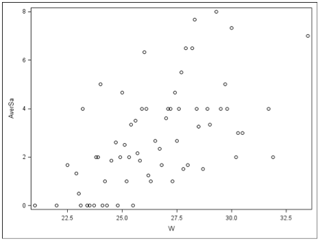
Plot of Average Number of Satellites by Width of Crab—Distinct Widths
|
 |
|
Plot of Average Number of Satellites by Width— Widths Grouped
|
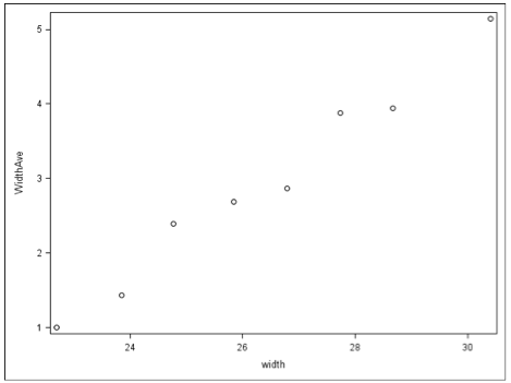 |
The data have been grouped into 8 intervals, as shown in the (grouped) data below, and plotted above:
    Interval  NumCases  AverWt  AverSa    SDSa    VarSa
      =23.25        14  22.693  1.0000  1.6641   2.7692
 23.25-24.25        14  23.843  1.4286  2.9798   8.8792
 24.25-25.25        28  24.775  2.3929  2.5581   6.5439
 25.25-26.25        39  25.838  2.6923  3.3729  11.3765
 26.26-27.25        22  26.791  2.8636  2.6240   6.8854
 27.25-28.25        24  27.738  3.8750  2.9681   8.8096
 28.25-29.25        18  28.667  3.9444  4.1084  16.8790
      >29.25        14  30.407  5.1429  2.8785   8.2858
Note that the "NumCases" is the number of female crabs that fall within particular interval defined with their width back. "AverWt" is the average back width within that grouping, "AverSa" is the total number of male satellites divided by the total number of female crab within in the group, and the "SDSa" and "VarSa" are the standard deviation that is the variance for the "AverSa".
Change the Model: Model the Rate Data
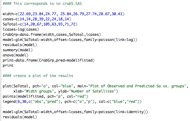
In the program below (see the last part of crab.r) we entered the grouped data above. In this case, each observation within a category is treated as if it has the same width.
We also create a variable lcases=log(cases) which takes the log of the number of cases (e.g, cases refer to the number of female crabs within particular group). This is our OFFSET that is the adjustment value 't' in the model that represents the fixed space, in this case the group (crabs with similar width). We thus form a rate of satellites for each group by dividing by each group size, and are fitting a loglinear model to rate of satellites incidence given the crab's width. "SaTotal" is the total number of male setellites corresponding to each grouping.
Here is the output.
Does the model now fit better or worse than before? It clearly fits better. For example the Value/DF for the residual deviance statistic now is 1.0861.
The estimated model is: $log (\hat{\mu_i}/t)$ = -3.535 + 0.1727widthi
As the width increases, the rate of satellites cases changes by exp(0.1727).
We can write the estimated model with respect to expected counts as: $log (\hat{\mu_i})$ = -3.535 + 0.1727widthi + log(t) where log(t) is the log(cases). For example, if we want to compute the estimated number of satellites for the second group of female crabs, $(\hat{\mu_1})$=exp(-3.535 + 0.1727x23.84 + log(14))=25.06 compared to 20 observed; see the plot below.
The residuals analysis indicates the good fit as well.

Let's compare the observed and fitted (predicted) values in the plot below:
This last two statements in R are used to demonstrate that we can fit a Poisson regression model with the identity link for the rate data. Notice that this model does NOT fit well for the grouped data as the Value/DF for residual deviance statistic is about 11.649, in comparison to the previous model.