12.7 - Population Structure
In human studies, but also in any study involving 'free living'animals, as opposed to laboratory animal studies, it is important to consider population structure.
Population structure occurs because individuals do not have access to the entire population to choose mates. In animal populations, and historically in human populations, individuals are more likely to have offspring with others who live nearby. Thus, even without considering sexual selection or survival of offspring, proximity induces assortative mating which makes certain SNPs more prevalent in each subpopulation simply due to the genotype of the founding population and genetic drift.
If we are looking at the phenotype of blonde hair and we have a mixture of individuals of both European background and non-European background, we will find many genes associated with European ancestry that are not necessarily causal for blonde hair. Similarly, there are many diseases that are more prevalent in some human populations than others. To understand the genetic components of these diseases, we need to distinguish between SNPs that are associated with the disease because they are more more (or less) prevalent in the population in which the disease is more prevalent and those that may have a causal link with the disease.
Take for example, type II (late on-set) diabetes. While diabetes is a problem in most human populations, it has higher prevalence in some groups, such as Native Americans. Disentangling the genetic and environmental causes of diabetes is quite difficult and is made more difficult by the fact that the same geographical isolation that created population genetic substructure also exposed the populations to different environments and led to different cultural traditions that might interact with the genetics to induce the disease.
Population substructure can often be determined using SNP data using a method called principal components analysis or PCA. We will discuss PCA in more detail towards the end of the course. For now, we just note that it is a means of finding several uncorrelated weighted averages of the features that have the greatest variance. We usually use the weighted averages to plot the data in 2 or 3 dimensions. We use all the data to find the weights for the weighted averages. We then use these weights to compute 2 or 3 different weighted averages for each sample.
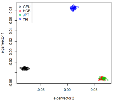 In the study shown at the right the following populations were involved:
CEU - Central European (Utah)
HCB – Han Chinese (Beijing)
JPT- Japanese (Tokyo)
YRI - Yoruba (Ibadan, Nigeria)
The SNPs were coded as 0,1 or 2 according to the number of "A" alleles. 2 weighted averages of the SNPs were computed - the first is the one with the maximum variance across the samples. Once the weights are computed, each individual gets a value (called the first principal component) by computing the weighted average using the SNP values for that individual. The second set of weights is computed so that the second principal component is uncorrelated with the first, and has maximum variance among the uncorrelated weighted averages. (This sounds complicated, but it is readily computed using matrix algebra.)
The plot shows each individual in the study plotted against the first 2 principal components and color coded by race. There is a very clear separation between the African, European and Asian individuals in this sample. The 2 Asian populations are not well separated - with just 2 principal components, but a 3rd component does separate them.
With this type of strong population structure, any study that includes individuals from all 4 populations is likely to have confounding due to the population structure. While you could study each population individually, you would likely get more statistical power by considering the subpopulation to be a block, and fit a generalized linear model similar to the model for the RNA-seq data. However, for SNP data we usually consider 0,1,2 to be ordinal and use ordinal logistic regression to fit a model with subpopulation as block and the phenotype as the predictor.

