Lesson 5: Microarray Preprocessing
| Key Learning Goals for this Lesson: |
|
Why Study Microarrays in the Era of High-throughput Sequencing?
Although nucleotide microarrays have competition from sequencing technology, they continue to be used for many purposes. As well, clever new types of microarrays continue to be devised, for example antigene microarrays. Nucleotide microarrays were the first high throughput method for genomics, introduced in 1995 [1]. Microarray data are intensities, which can be treated as continuous data. By using the log2 transformation, the data are suitable for analysis by enhanced versions of standard statistical methods such as t-tests and ANOVA, which are taught in introductory statistics courses. Sequencing data are counts, which require more difficult statistical models which might more simply be viewed as extensions of these methods. So, from the pedalogical viewpoint, microarray data analysis provides a simpler setting in which the statistical issues common to all high throughput biological data can be discussed. Finally, many legacy microarray data sets are publicly available; these can and should be used to support current studies using other technologies. Often the data need to be re-analyzed for this purpose.
What is a Microarray?
A microarray is a glass or plastic slide or a bead that has a piece of DNA or cDNA (an oligonucleotide or oligo) attached to it. For genomic resequencing, such as genotyping, the oligos will be pieces of DNA; for gene expression it would be cDNA derived from the transcripts.
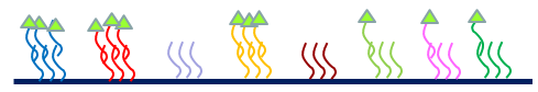
In the diagram below you can see a labeled sample and the complementary probes that are on the substrate. Both the sample and the probes are single strands, and hybridization proceeds by binding of the sample strands to the complementary probes on the array.
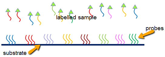
The probes should capture only the complementary strands from the sample (although cross-hybridization does occur).
After hybridization the microarray is washed to get all the loose labelled nucleotides off and then we put the whole thing through a scanning microscope at each label wavelength. The intensity of the dye is expected to be proportional to the amount of labeled material in the sample for each probe. Since both hybridization and labeling are chemical processes, we know that binding is affected by the energetics of the system, so that two different types of strands with the same concentration may not label and hybridize equally. However, we expect that the same type of strand should label and hybridize equally well in different sample. i.e. we can compare intensities for each feature across microarrays more reliably than we can compare different features on the same microarray.
What is a micro array probe?
Each probe of the microarray is a set of lots identical strands of DNA that are supposed to be complementary to what is in the sample. The DNA is synthesized from known sequences. We may not know what feature they represent, but we have the genomic sequence.
Microarray Quantification
The primary data is a digital black and white photograph of the array. For two channel microarrays arrays which have two differently labeled samples hybridized to the same probe, the data are often visualized by a picture like the one below. This is actually a composite of the black and white photo for each label. One of the labels is represented by red and the other by green. The relative intensity of the two samples is represented by a color scale going from pure red (only the red sample has hybridized) to pure green (only the green sample has hybridized) with yellow meaning equal amounts of both samples. The intensity is represented by brightness, so that dark spots show little hybridization and bright spots have high hybridization.
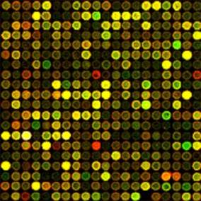
This is a very old picture. The probes on modern microarrays are much more uniform and show up as perfect circles.We don't really use the visualization except for quality control, as the quantification is done on the individual grayscale photos.
Quantifying Probe Intensity
The software that comes with the scanner locates the probe centers, radii and also determines what should be considered the local probe background.
To obtain a summary for the probe we need to identify
- The pixels in the probe foreground - i.e. the region which has the complementary strands.
- A probe summary such as the mean or median.
- The pixels in the background.
- A probe summary for the background
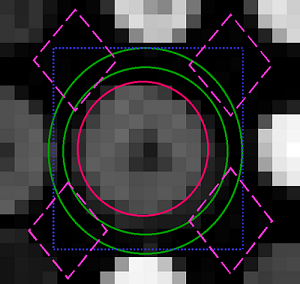
In the picture above, the probe foreground is inside the red circle. There are various ways of defining the background. One method is to use the annulus between the green circles. Another method uses the 5 pink rhomboids.
There are many pixels enclosed in both the foreground and background. Usually a single summary is used for each. For the foreground, it is considered important to avoid outliers, so the median or a trimmed mean are often used. For the background, a similar summary or the pixel mean can be used.
The remaining details vary by microarray type. There are 3 main types: low density oligo arrays (which are the modern version of the original "spotted" arrays), high density oligo arrays, and bead arrays. This last type is seldom used at Penn State and will not be discussed in this class. However, the general principles are the same for all the types - the difference with bead arrays is that the probes need to be identified, whereas on oligo arrays the probes are printed on fixed locations on the array surface.

