Printer-friendly version

Bootstrapping is a method of sample reuse that is much more general than cross-validation [1].  The idea is to use the observed sample to estimate the population distribution.  Then samples can be drawn from the estimated population and the sampling distribution of any type of estimator can itself be estimated.

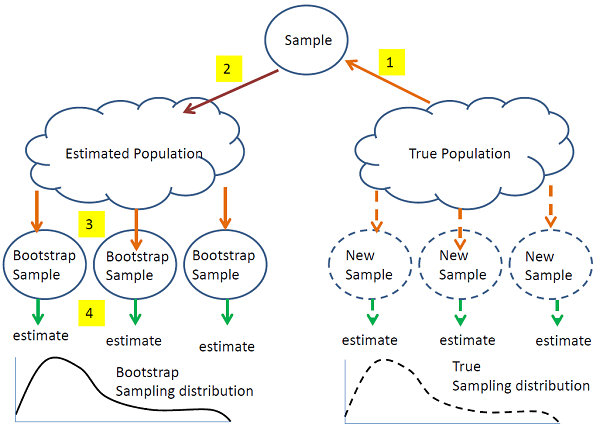
The steps in bootstrapping are illustrated in the figure above.  Observed quantities are denoted by solid curves and unobserved quantities by dashed curves. The objective is to estimate the true sampling distribution of some quantity T, which may be numeric (such as a regression coefficient) or more complicated (such as a feature cluster dendrogram).  The true sampling distribution is computed by taking new samples from the true population, computing T and then accumulating all of the values of T into the sampling distribution.  However, taking new samples is expensive, so instead, we take a single sample (1) and use it to estimate the population (2).  We then (3) take samples "in silico" (on the computer) from the estimated population, compute T from each (4) and accumulate all of the values of T into an estimate of the sampling distribution.  From this estimated sampling distribution we can estimate the desired features of the sampling distribution.  For example, if T is quantitative, we are interested in features such as the mean, variance, skewness, etc and also confidence intervals for the mean of T.  If T is a cluster dendrogram, we can estimate features such as the proportion of trees in the sampling distribution than include a particular node.

There are three forms of bootstrapping which differ primarily in how the population is estimated. Most people who have heard of bootstrapping have only heard of the so-called nonparametric or resampling bootstrap.

• Nonparametric (resampling)
• Semiparametric (adding noise)
• Parametric (simulation)

Nonparametric (resampling) bootstrap

In the nonparametric bootstrap a sample of the same size as the data is take from the data with replacement. What does this mean? It means that if you measure 10 samples, you create a new sample of size 10 by replicating some of the samples that you've already seen and omitting others. At first this might not seem to make sense, compared to cross validation which may seem to be more principled. However, it turns out that this process actually has good statistical properties.

Semiparametric bootstrap

The resampling bootstrap can only reproduce the items that were in the original sample.  The semiparametric bootstrap assumes that the population includes other items that are similar to the observed sample by sampling from a smoothed version of the sample histogram.  It turns out that this can be done very simply by first taking a sample with replacement from the observed sample (just like the nonparametric bootstrap) and then adding noise. 

Semiparametric bootstrapping works out much better for procedures like feature selection, clustering and classification in which there is no continuous way to move between quantities. In the nonparametric bootstrap sample there will almost always be some replication of the same sample values due to sampling with replacement.  In the semiparametric bootstrap, this replication will be broken up by the added noise.  

Parametric bootstrap

Parametric bootstrapping assumes that the data comes from a known distribution with unknown parameters. (For example the data may come from a Poisson, negative binomial for counts, or normal for continuous distribution.) You estimate the parameters from the data that you have and then you use the estimated distributions to simulate the samples. 

All of these three methods are simulation-based ideas.

Examples

Clustering

The nonparametric bootstrap does not work well because sampling with replacement produces exact replicates. The samples that are identical are going to get clustered together. So, you don't get very much new information.

The semi-parametric bootstrap perturbs the data with a bit a noise.  For clustering, instead of taking a bootstrap sample and perturbing it, we might take the entire original sample and perturb it.  This allows us to identify the original data points on the cluster diagram and see whether they remain in the same clusters or move to new clusters.

Obtaining a confidence interval for a Normal mean (a parametric example)

Suppose we have a sample of size n and we believe the population is Normally distributed.  A parametric bootstrap can be done by computing the sample mean \(\bar{x}\) and variance \(s^2\).  The bootstrap samples can be taken by generating random samples of size n from N(\(\bar{x},s^2\)).  After taking 1000 samples or so, the set of 1000 bootstrap sample means should be a good estimate of the sampling distribution of \(\bar{x}\).  A 95% confidence interval for the population mean is then formed by sorting the bootstrap means from lowest to highest, and dropping the 2.5% smallest and 2.5% largest.  the smallest and largest remaining values are the ends of the confidence interval.

How does this compare to the usual confidence interval: \(\bar{x}\pm t_{.975}s/\sqrt{n}\)?  Our interval turns out to approximate \(\bar{x}\pm z_{.975}s/\sqrt{n}\) - that is, is uses the Normal approximation to the t-distribution.  This is because it does not take into account that we have estimated the variance.   There are ways to improve the estimate, but we will not discuss them here. 

Obtaining a confidence interval for  \(\pi_0\) with RNA-seq data (a complex parametric example)

For an example of using the parametric bootstrap let's consider computing a confidence interval for  \(\pi_0\) an RNA-seq experiment. In this case we will assume that the data are Poisson. Here is what we would do:

1) First we estimate \(\pi_0\) from all of the data.

2) Now we need to obtain a bootstrap sample from the Poisson distribution.  We will hold the library sizes fixed.

a) For each treatment:

i) in each sample for each feature, recompute the count as the percentage of the library size.

ii) for each feature compute the mean percentage over all the samples from that treatment - call this \(g_{i}\) where i is the feature.

iii) For each sample,  multiply the library size \(N_j\) where j is the sample, by \(g_i\) to obtain \(N_jg_i\) the expected count for feature i in sample j.

iv) The bootstrap sample for feature i in sample j is generated as a random Poisson with mean  \(N_jg_i\) .

b) Now that there is a bootstrap "observation" for each feature in each sample, redo the differential expression analysis and estimate \(\pi_0\).

c) Repeat steps a0 and b0 1000 times. Now you have 1000 different estimates of \(\pi_0\) - this is your estimate of the sampling distribution of the estimate.

3) Your 1000 bootstrap estimates can be used to draw a histogram of the sampling distribution of the estimate of \(\pi_0\).  The central 95% of the histogram is a 95% confidence interval for  \(\pi_0\).  To estimate this interval, it is simplest to use the sorted bootstrap values instead of the histogram.  For example, if you drop the 2.5% smallest and largest values, the remainder are in the 95% confidence interval. To form the ends of the interval, use the smallest and largest of this central 95% of the bootstrap values.

This is a parametric bootstrap confidence interval because the bootstrap samples were generated by estimating the Poisson means and then generating samples from the Poisson distribution.

[1] Efron, B. (1982). The jackknife, the bootstrap, and other resampling plans. 38. Society of Industrial and Applied Mathematics CBMS-NSF Monographs. ISBN 0-89871-179-7.