15.5 - Aggregated Prediction
Bootstrapping was developed around 1982. Around 1994, the idea of using the bootstrap samples to improve prediction was proposed [1,2 ]. Bootstrap aggregation (shortened to "bagging") computes a predictor from each of the bootstrap samples, then aggregates into a consensus predictor by either voting or averaging. Random forest is a similar method using classification trees.
Example
This example comes from an observational study of cardiovascular risk. We cannot randomly assign people to low and high risk environments. One interesting design is to study populations in which originate in low risk environments but migrate to high risk environments. These data come from a study of Peruvian Indians moving from the high lands of Peru (low risk) into a major city (westernized diet and lifestyle leading to higher risk). The researchers measured a bunch of physical attributes that are thought to be related to cardiovascular disease:
- Age,
- Years (in city),
- Height,
- Pulse,
- Systolic BP, and
- 3 skinfolds: Chin, Forearm, Calf
The three skinfold measurements are a measure of fat under the skin and are highly correlated with one another and with weight. This high correlation causes problems in prediction, so often variable selection is used to pick the features that are the good predictors.
Bagging - Aggregating multiple linear regression with variable selection
Multiple linear regression was used to develop a measure of weight predicted from all of the other variables. Variable selection (stepwise regression) was used to select a smaller set of predictors, because of the problems of high multicollinearity of the predictors.
Now lets see how bagging would work for this example. A large number of nonparametric bootstrap samples were taken from the data. For each bootstrap sample variables were selected using stepwise regression and from this a multiple linear prediction equation was created to predict the weight of all the individuals (including those not selected in the bootstrap sample). Bagging was done by averaging the predictions across all the prediction equations and is shown in black in the plot below. For comparison we also predicted the weight using all the other variables, shown in red on the plot.
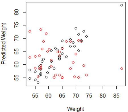
You can see that the red predicted weights are not well correlated with the true weight, while the bagged predictions are highly correlated.
As well, the bagged estimated come with some bonus uncertainty assessments. For each individual in the study, each of the bootstrap samples gives us a prediction. Therefore if we delete the 2.5% smallest and largest values, we have 95% confidence interval for individuals with the same measurements that does not rely on Normality assumption.
As well, we can assess how important each of these variables is as a predictor by counting how many times each variable was selected.
| Age | Calf | Chin | Forearm | Height | Pulse | BP | Years |
| 773 | 372 | 848 | 862 | 1000 | 194 | 993 | 945 |
Height always got selected - this is not surprising because taller people tend to be heavier. On the other hand some of the information is surprising. For example, pulse is not selected often, but blood pressure is, suggesting a correlation between weight and BP in this group. Calf skinfold is only selected about 1/3 of the time - this might suggest a lack of correlation between calf skinfold and weight, or it may be due to the multicollinearity with the other skinfold measures. In any case, these counts might give a researcher some important clues about the epidemiology of questions under consideration.
Random Forest
Although a method called regression trees can be used similarly to classification trees for prediction, we will focus on classification. (The random forest idea can be used with regression trees very similarly to bagging.)
Suppose that each individual is classified into Normal or overweight based on their body mass index (weight/height2) over or under 25. (There is also an obese category - over 30, but there is only one individual in this sample in this category.) We then use recursive partitioning to classify the samples into these two classes, using all of the variables except for weight. We obtain the following tree:
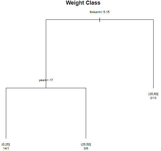
Next we bootstrap, creating a tree for each bootstrap sample. This is called a random forest. Each observation is classified by each tree and the final classification is by majority rule.
Here are the two confusion matrices:
Recursive partitioning (without bootstrapping)
                     true class    Normal        Overweight
predicted
                   Normal          14                   1
                   Overweight       5                  19
Random forest
                     true class    Normal        Overweight
predicted
                   Normal          15                   6
                   Overweight       4                  14
In most cases, random forest is a better classifier, but this example is one of the exceptions. It is not clear why, but it might be due to the sharp cut-point used for BMI, as 1/3 of the sample has BMI between 24 and 26.
References
[1] Breiman, Leo (1996). "Bagging predictors". Machine Learning 24 (2): 123–140. doi:10.1007/BF00058655. CiteSeerX: 10.1.1.121.7654
[12] Breiman, Leo (2001). "Random Forests". Machine Learning 45 (1): 5–32. doi:10.1023/A:1010933404324

