6.1 - Two Condition Studies
The most basic differential expression study has two conditions. These could be:
- treatment vs control
- mutant vs wild type
- exposure B versus exposure C
The first thing we will do is look at how this works on a two channel microarray. Because we find that the two channels on the same microarray are more similar than samples on different microarrays, we will used a paired analysis. Usually each array will have both conditions using a dye swap design. The dye effect will average out over the arrays, as long as the same number of samples for each treatment are labelled with each dye, so we do not need to create a special statistical model with a dye effect. However, M=log2(R)-log2(G), so for some microarrays M represents B-C and for others C-B and we do need to keep track of that.
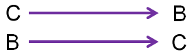
For the colonCA data, let's assume that the 22 paired samples were paired on the arrays (i.e. the two tissues from the same subject were hybridized to the two channels on the same array) and that red is always reported before green. (When we have data from a lab or a data repository, it should be clear which samples are labeled with each dye.) There is a positive patient number for the normal tissue samples and a negative patient number with the same number with for the tumor tissue samples. This makes it easy for us to look at the data.
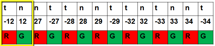
For example, we can see below that the first two columns are microarray 12 with the tumor in the red and the normal in the green.
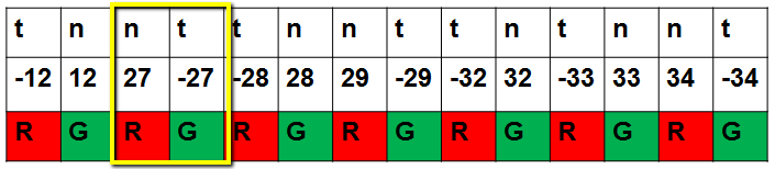
For microarray 27 (columns 3 and 4), the normal is in the red and the tumor is in the green. This is exactly what we expect in a dye-swap design.
Typically, the data will be arranged in two matrices, one for the red channel on each array, and one for the green, as shown below. After normalization, we obtain M=log2(R)-log2(G). For the paired comparison, we reduce the data to d=log2(normal)-log2(tumor) for each patient (microarray). As shown below, on array 12, d=-M and on array 27 d=M.
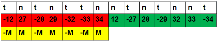
To account for this, we make a "design matrix" which is a matrix with one column and 22 rows (one for each microarray). The entry is +1 if d=M and -1 if d=-M, so that the element-wise product of the design matrix and the M values is d. This simple operation allows us to compute the d values associated with every gene in a single matrix operation, giving us a matrix of the log2 expression difference between normal and tumor for every gene on every microarray as a matrix with genes in the rows and microarrays in the columns.
We can then compute the t-statistic for each row, giving us a paired t-test for every gene. Some of the t-statistics are shown below, along with the histogram of all of the 2000 t-statistics. If there is no differential expression, these t-statistics all come from the null distribution. Assuming that the difference in log2 expression values is approximately normal, the null distribution should be t with 21 d.f. for each of the genes.
| Hsa. 3004 | -2.057516 | 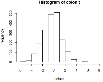 |
| Hsa.13491 | -1.169676 | |
| Hsa.13491.1 | -1.590321 | |
| Hsa.37254 | 1.137496 | |
| Hsa. 541 | -1.750747 | |
| Hsa. 20836 | -0.851902 |
The results look fairly bell-shaped, but there might be some genes with t-statistics farther out in the tails than expected. To be sure, we need to compute the p-value for each test, based on the t on 21 d.f. as the reference null distribution.
Instead of computing a t-statistic for every gene using a loop, we will use the LIMMA package, which computes the mean difference and the s.e. of the mean difference efficiently using matrix operations. We will use the LIMMA package throughout this course.
Here are the results that we get using LIMMA.
| t.test | LIMMA (unmoderated) | |
| Hsa. 3004 |
-2.057516 |
-2.057516 |
| Hsa.13491 | -1.169676 |
-1.169676 |
| Hsa.13491.1 | -1.590321 |
-1.590321 |
| Hsa.37254 | 1.137496 |
1.137496 |
| Hsa. 541 | -1.750747 |
-1.750747 |
| Hsa. 20836 | -0.851902 |
-0.851902 |
One reason to use LIMMA is computational efficiency. ColonCA has only 2000 genes, so computing the t-statistic using a loop does not take very long. However, when we have 30 - 60 thousand genes, using a loop is quite slow. However, LIMMA has two other advantages. It turns out that the idea of using a design matrix allows for very flexible statistical analysis. Be changing the design matrix, we can use LIMMA for complicated experimental designs like 2-way ANOVA and randomized complete block designs. We can have a mix of paired and unpaired samples. We can do analysis of covariance (ANCOVA) or regression. As well, the default method in LIMMA uses an empirical Bayes estimate to "moderate" the standard deviation in the t-test denominator using the distribution of all the standard deviations. This can really improve the power especially with small samples. Recall that although power is the probability of correctly rejecting the null hypothesis when it is false, if we obtain more power for the same p-value then we actually improve the false discovery rate as well.
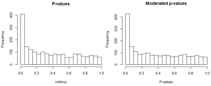
Below are the p-values from the 2000 paired t-tests using the ordinary t-statistic and the moderated t-statistic. Because our sample size (22) is relatively large, there is not a huge difference between the two test statistics, although if you look carefully you can see that the first bin is slightly higher for the moderated test (which is what you expect if there are some truly differentially expressing genes).
The table below shows the estimated percentage of genes that do NOT differentially express \(\pi_0\)
|
Pounds and Cheng \(\pi_0\) |
Storey \(\pi_0\) | tests with p < 0.05 | |
| ordinary t | 0.758 | 0.664 | 122 |
| moderated t | 0.761 | 0.679 | 178 |
Pounds and Cheng's method says that about 25% differentially expressed and about 75% don't. Storey's method says that roughly 33% differentially expressed. However, both methods estimate a slightly larger percentage of NON-differentially expressing genes using the moderated test. And yet, at p<0.05, there are almost 50% more "detections" using the moderated test. Why?
The moderated t has more power so there are fewer non-detections. Even the most conservative of the 4 estimates of \(\pi_0\) estimates that 25% or 500 genes differentially express. So, even if we reject at p<0.05 and ALL the discoveries are true, we have a substantial number of false nondiscoveries. The moderated method improves power and so reduces the false nondiscovery rate by using information from the population of genes to improve the estimate of the SD of expression for each gene.
What is a Moderated T-test?
The idea of moderation comes from a deep and surprising statistical result called Stein's paradox [1]. In its simplest form it states that when you are estimating 4 or more population means, the best estimator is not the 4 or more sample means, but a weighted average of the sample means and the "mean of the means". One way to find an appropriate weighting is to assume that the population means themselves come from a population (which is a Bayesian idea). This population is then the prior, and the best estimator of each population mean is the Bayes predictor, which is a weighted average of the prior mean and the sample mean. LIMMA uses an Empirical Bayes method which estimates the prior from the set of all feature(since we have 2000 of them - one for each gene).
LIMMA uses this Empirical Bayes method to moderate the sample variances, which are mean squared deviations (and so are a type of sample mean). Below is a plot of variance of the genes and beside it a gamma distribution with the mean and variance matching the average of variance of the sample variances. (Got that? We computed 2000 variances and then used them as a sample to compute a mean and variance.)
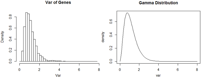
The shapes of these two plots is very similar (although the peak of the Gamma distribution is slightly lower.) LIMMA assumes that the variances come from a Gamma distribution and uses the variances computed for each gene to obtain the empirical estimates of the mean and variance of the Gamma. This Gamma distribution is the empirical prior distribution for the variances.
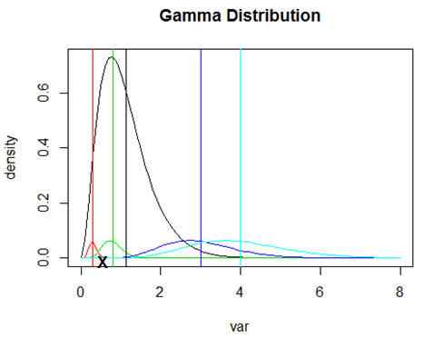
Now consider the plot below of the same Gamma distribution. The mean of the distribution is denoted by the vertical black line. The other 4 vertical lines are the TRUE (but unknown) variances of 4 genes. The curves of the same color are the sampling distributions of the sample variances for sample size 22 for a gene with this variance. Notice that the genes with high variance have a sampling distribution that is very spread out and that there are a lot of sample variances in the left tail. So, if we observe a gene with a large sample variance, its true variance is likely to be smaller. Conversely (and harder to see on this plot) the genes with variance smaller than the mean variance are have more sample variances below the true value. The moderated variance is a weighted average of the black line and the observed variance for each gene. This pulls the large variances down towards the mean variance (making the t-tests for those genes more powerful) and the small variances up towards the mean variance (making the t-tests for those genes less powerful). Moderation is somewhat like having a larger sample size for estimating the variance because the sample variance (on average) is more likely to be far from the population variance, while moderated variances are (on average) closer. The moderated variance also has an associated d.f. that is higher.
This empirical Bayes moderation turns out to be equivalent to having a larger sample size. So, as well as shrinking the sample variances towards the mean variance, the associated degrees of freedom increase. These are the d.f. of the null t-distribution for the moderated t-test. Recall that as the d.f. of a t-test increase, the critical values decrease. Using the moderated variance to estimate the SD has two effects on the t-test - the SD in the denominator of the test changes and the d.f. increase. The result is that for genes with large sample variance, power is increased in two ways - the moderated sample variance is smaller and the d.f. are larger. For genes with small sample variance, power is decreased by having a larger moderated sample variance and increased by having more d.f.
If you had a sample size of 100 instead of 22 all of the distributions would be narrower, and there is less shrinkage. As a result, the amount of moderation adjusts automatically to the amount of information available for each gene.
In summary, the moderated t-test is a t-test using the square root of the moderated variance as the SD instead of the sample variance. Having a better estimate of the standard deviation in turns out to be reflected in having more power for the tests. You would have the most power for that sample size if you actually knew the standard deviation, in which case you would use a normal distribution for the null distribution.
There are many different models for doing variance moderation: Cyber T and SAM are two of these products available in R which use moderated variances with a somewhat different justification. I prefer LIMMA and the associated statistical model because the clever empirical prior used by LIMMA leaves us with t-tests. Using other software you have to simulate to get the null distribution. Using LIMMA means that the t-test using the moderated standard deviation continues to have a t-distribution when the null is true, but there is a change in the d.f. associated with the moderated variance which is computed along with the moderated standard deviation. Simulations done by Smyth and others confirmed that the moderated t-test gains power. This means that the for any given false discovery rate, the false non-discovery rate will be smaller.
Doing the moderated tests with LIMMA
To perform the moderated tests with LIMMA we start with the normalized data. For two-channel microarrays, we usually use the normalize M as the data, which will give us a moderated paired t-test. This is appropriate, because hybridizing the two samples on the same microarray induces a pairing. As well, for the colonCA data, we have assumed that the two samples on the same array are also from the same patient.
We require a "design matrix" to determine what needs to be averaged for the test. When there are dye-swaps, some M values are B-C and others are C-B, so our design matrix is a single column of +/-1 with +1 for Normal-Cancer and -1 for Cancer-Normal. Denoting the design matrix as D and the column of M values as M, DTM is the average Normal-Cancer value.
Given the data and the design matrix, LIMMA computes the difference in means the the appropriate SD in the one step, and then computes the moderated SD and the moderated t-test in the "eBayes" step. I then usually use Storey's method to compute q-values and come up with a final gene list.

