Printer-friendly version

In this section, we work with independent samples. We assume that the measurement platform is a 1-channel microarray such as an Affymetrix array, or a two channel 'reference design'in which one channel is devoted to a reference sample, so that M=sample-reference.  We start with normalized data on the log2 scale, in a data matrix with genes in the rows and samples in the columns.   

We will use the colonCA data again, but this time we use only the normal samples from the 22 patients with two samples, and only the cancer samples from the 18 patients that had only cancer samples.  This gives us independent samples.

Our typical situation is that each sample is on separate array and the analysis will be a two sample t-test. Again, we can do this by doing t-tests for every row. But we prefer to do the empirical Bayes or 'moderated' t-test because to get a little more power.

In the paired case, we had an M value for each patient which represented the difference in expression, so our design matrix required only one column which gave the sign of M.  In the unpaired case, some patients provided cancer samples and others provided normal samples.  So we need a slightly different design matrix.  I prefer to use what is called the treatment means model.  The columns of the design matrix are indicator variables for each treatment group.  So, in this case, we have 2 columns.  One column has a 1 for each normal sample and a 0 for each tumor sample, while the other column has a 1 for each tumor sample and a 0 for each normal sample.  Letting D be the design matrix and E the log2(Expression) matrix (after normalization) we find that M=ED is a 2000 x 2 matrix.  The first column is the sample mean for the normal samples for each gene and the second column is the sample mean for the tumor samples for each gene.  The ordinary (unmoderated) variances are the pooled within treatment variances.

To obtain the difference in means, we use a contrast matrix.  If C=[1,-1] a 1x2 matrix, then MC^T is a 1x2000 matrix with the difference in means for each gene.  

In the final step we moderate the pooled within variances exactly as we did in the paired case, and compute the moderated two-sample t-statistics (using the pooled variances).  

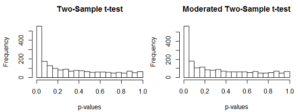
Below you can see the 2000 p-values from the usual two sample t-tests and a moderated two sample t-test.  As we saw with the paired t-test, the moderation does not have a large effect, because the samples sizes (18 and 22) are relatively large.  But we do expect some additional power due to the moderation.

As we did before, we also estimated \(pi_0\), the percentage of genes that do not differentially expressed. We used the Pounds method which is the average p-value. We also use the Storey's method which uses the the area under the flat part of the curve. They are somewhat different but both show that there is quite a bit of differential expression. At most 65% of the genes do not differentially express and 35% do. As before, our nondetection rate is pretty high, since we expect about 35% of 2000 = 700 genes to differentially express.  And, as before, we detect more "significant" genes with the moderated than with the unmoderated test, even though the estimate of \(\pi_0\) is quite similar.

So far we have done two different analyses (paired and unpaired), each using part of the data.  The power of LIMMA and other "linear models" methods is that we can fit a model that uses all the data.  We will look at that in Chapter 7.