Printer-friendly version

Affymetix@ was a pioneer in using print technology to synthesize oligos and the microarray surface.  This enabled them to print very high density microarrays that were originally more accurate (and more expensive) than the low density arrays.  The basic paradigm is that use of multiple oligos for each gene provides a more stable estimate of gene expression.  As well, the basic idea extended readily to genotyping microarrays (which are still heavily used and much cheaper than genotyping by sequencing).  Although newer printing technologies and sequencing are now competitive with Affymetrix microarrays for gene expression, these arrays are still frequently used, especially for model species.  As well, because these microarrays provided good quality data as early as 2001, the historical data is still useful for planning and comparison purposes. 

Because of the popularity of these microarrays, a number of special quality control and normalization methods were designed specifically for them.  Some of these methods are also used with lower density microarrays which have multiple probes per gene (i.e. a probe set).  The main differences between Affymetrix and other multi-oligo arrays (from the statistical viewpoint) is that Affymetrix arrays use 9 - 16 short (25 base) oligos to represent each gene.  The lower density multi-probe microarrays typically have fewer, but longer oligos.

Affymetrix Features

The older Affy arrays have what are called perfect match and mismatch probes. A PM (perfect match) probe matches to the annotated reference at the time the array was created. The corresponding MM (mismatch) probe differs from the PM by a change in the central nucleotide. The idea was that this would measure the 'noise' and cross-binding from similar genes.  

On the older gene expression microarrays, the PM probes are biased to the 3' end of the gene.  This was to enhance uniqueness, as well as reduce bias due to mRNA degradation.  There are a number of known problems - wrong annotations, probes which do not hybridize well, and missing expression when splice variants do not cover the probes.  While it is possible to correct for these problems, this is seldom done except for comparison with other platforms.  Using the microarrays "as is" allows for comparison with older datasets.

The MM probes were originally supposed to provide additional background correction.  This proved unsuccessful, and the MM probes were dropped from later microarrays.  There is a normalization (MAS5) that uses the MM probes - the main use of this method currently is to determine the lower detection limits of the probes, as the MM probes can be used to provide evidence of "signal above background".  Fortunately, the MM idea was perfect for SNP microarrays, and Affymetrix has faired well in the genotypying world.

This sketch from the Affymetrix website shows the probes on the 3' of the gene, illustrating PM and MM oligo selection.

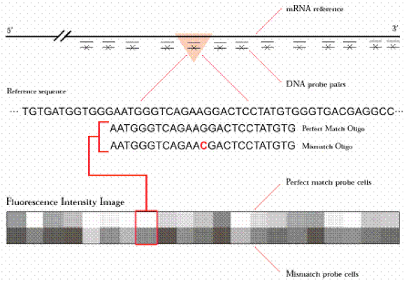
image of Oligonucleotide Probe Pair from Affymetric

The newer microarrays were annotated to updated genomes and transcriptomes and have more even coverage of the transcripts.  As well, the gene expression arrays do not have MM probes.  

Among the many reasons that Affymetrix microarrays have maintained their popularity is that the probes are completely annotated with both sequence and location in the genome, as are cross-annotated to other popular annotations such as RefSeq.

Quality Control

As with other microarrays, I usually start my quality control efforts with graphics.  The first graphic is a surface plot, showing the intensity of each probe on the array surface. These often appear streaky.  As well, the array id and some control probes are printed on the array surface and can usually be seen on the plot.

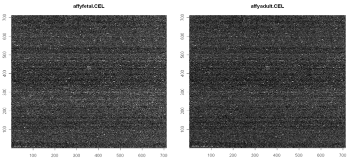
I like the red/yellow color scheme, which makes it easier to detect features.  A solid red band appears at the top or bottom of the image if the probes do not take up the entire surface.

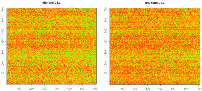
If you see blobs, or streaks that are not horizontal, there might be problems with the array.  There are some more delicate tools that fit spatial loess and then look at the residuals.  These can find more subtle problems with the arrays if this seems necessary.  There are a number of packages in Bioconductor which do various probe-level analyses, including quality control analysis.  

I also plot the log2 of the raw probes against each other:

These plots you usually look like this if the arrays are good quality. Remember, you will have between nine and 16 probes from the probe set and the normalization usually downgrades outlying probes, so a few unusual probes shouldn't really trouble you.

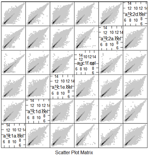
Next is an example from a miRNA array study.

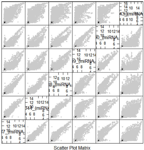
The microarray that is at the top and right of this plot is more spread out than the others, and also seems to have a lot of low-expressing probes.  There is really something wrong with this array. This study only has six arrays so one bad microarray can affect the conclusion. We didn't notice it originally because micro array facility that created the slides did quantile normalization on the data. Once they went through this normalization all the microarrays looked the same.

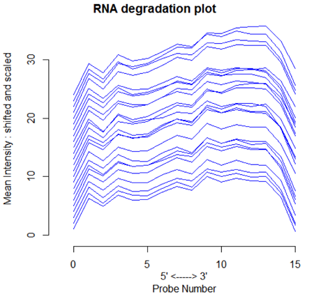
Another thing that we can do, mostly because it's convenient in R, is called the RNA degradation plot. The original idea was to check the quality of the sample for RNA degradation, using the fact that degradation proceeds from the 5' to the 3' end.  Since each probe in the probesets are numbered by location, averaging over probe 1, probe 2 etc for all the probesets gives a snapshot of the average intensity by a rough measure of 5'-ness.  It was expected that good samples would be flat.  I have not seen this.  However, when the microarrays are good, they all have the same pattern, like the plot below. 

In the RNA degradation plot below, we can also see that the mean level of the probes differs among the microarrays.  This is an indication that normalization is necessary.

Finally, I have seen a situation in which all of the RNA degradation plots for each treatment were similar but differed from the plots for the other treatment.  This might indicate that one treatment is inducing some type of RNA degradation.  If all the plots from one lab are similar but differ from those from another lab, that would indicate that there are systematic lab biases that need to be accounted for in the analysis.

One thing that was of great surprise to a lot of people originally,  is that probes in a probe set do not all give you the same expression level. This also occurs in RNA-seq, where we expect, but do not see, even distribution of reads across a transcript.   On the plots below we have the observed expression level for all the microarrays in the study for 4 probesets (natural scale).  We can see that the expression levels differ greatly, and so does the array to array variability.  The variability is greatest where the maximum expression is greatest (check the y-axis to see this).

.  

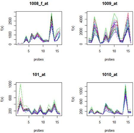
When this was first observed, it was thought that perhaps the low intensity probes were poor - possibly mistaken annotation or poor binding.  However, from the RNA-seq data we can see that there might also be other explanations, such as the pattern of fragmentation of the transcripts during sample preparation.

Since there are about 20,000 probesets on an Affymetrix microarray, we usually do not do the plot of expression by probe for every probeset.  However, this might be of interest if you were interested in particular genes.

Over all, the arrays are assumed to be of good quality if they show similar patterns.

Data Extraction

The raw Affymetrix data is stored in what is called a CEL file.  The CEL file has the probe id, probe location and probe intensity for each probe, as well as information which identifies the type of array.  (The identifier is used to find the annotation which links the probes to their probeset and the probeset to the gene id.)

CEL files come in 2 formats - a regular text format which can be read by a text editor or Excel, and a binary format which needs a decoding step.  The Bioconductor package affy can read the files in either format, which saves us the trouble of having to identify the file format.

Once the data have been read into the affy software, we need to do background correction, probe normalization and finally summarization of the probes into probesets. We are going to look at methods for gene expression microarrays. miRNA arrays, SNP arrays, etc. might require different methods.

Normalization and Summarization

Normalization of Affymetrix microarrays was an active research area for about 10 years.  Affymetrix created 2 benchmark experiments that researchers could use to test their methods, and there was a website where bioinformatics researchers could upload their software and subject their method to a competitive test.  The affy  software includes several of these methods and also allows the user to "mix and match" picking different background correction, probe normalization and probeset summary methods.   However, for publication purposes, it is usually best to select one of the standard methods.  Of these, the most used appears to be RMA.

Robust Multi-array Analysis (RMA)

The method that we will talk about here, robust multi-array normalization is meant for gene expression microarrays, but is also used for some other types of microarrays . RMA covers all 3 steps - background correction, quantile normalization of the individual probes and then probeset summary.  

Background correction is done using a fairly complex statistical model which supposes both additive and multiplicative noise components.  After background correction to the individual probes, quantile normalization is applied.

In the final step, the probes are summarized into probesets using the median polish algorithm, which is a type of robust 2-way ANOVA, where one factor is the array and the other is the probeset.   The algorithm is robust to outlying data, so that single probes with large values are down-weighted.  Because both quantile normalization and median polish use data from all the microarrays, using just a subset of the microarrays or removing a single bad array affects the normalization step for all the arrays.

For the median polish algorithm, we consider the matrix consisting of the probes in the columns and microarrays in the rows.  We start by taking the median of each probe across the microarrays - that is the probe effect.  We remove the probe effects from each column by subtraction giving a residual.  We then take the median of the residuals across the probes - that is the array effect.  We do this iteratively until there is no change, and then add up the effects.

For example, if we have three arrays and five probes the first thing we do is to find the median across the array (values in the yellow row). Then, this is subtracted off to give you the value in the top row of the next table.

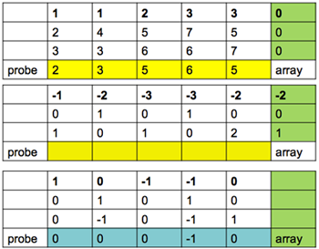
Next, will find the median in the opposite direction for the array. And subtract this off to give us the values in the top row of the third table.

When you subtract all of these values what you see is that the only column that changes is, because of the zero is the one on the right.

Next you add up the margins to get the array effect for this gene and probe set effect for the array.

array -2, 0, 1

probe 2, 3, 5, 5, 5

For each array the summary is the sum of the probe set effect and the array effect.

probe median = 5
probe + array = 3, 5, 6 (the expression of the gene on arrays 1, 2, 3)

This method is a bit complicated but it is robust to outliers.

RMA is probably the most popular normalization.  A related method, GCRMA does a GC bias correct step after background correction and prior to quantile normalization.  It requires quite large sample sizes and has been used primarily with human microarrays.

Two other popular methods are dChip and PLIER.  The original method, MAS5, has been shown to be less effective; as well, it uses the MM probes, which are not printed on the newer models of microarrays.

Does the Normalization Matter For Assessing Differential Expression?

It would be nice if the different normalization methods differed only for a few genes, but unfortunately, results can differ substantially, especially for small studies.  Below is a scatterplot matrix of one CEL file with different normalizations (including probeset summary).  The large differences in the probeset summaries translate to even larger differences in differential expression estimates. 

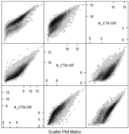
One of the things that you might find it shocking is that the overlap in the genes that were declared differentially expressed, from the exact same microarrays, was only 50% no matter whether one considered the top 25, top 50 or 100 genes.  Since different statistical analyses give very different lists of genes, for biological inference we are going to need to add other sources of information.

When you are comparing your data with previous studies, you should use the same normalization. You should always keep your raw data and for replicability you should always include in your paper how you did the normalization. The supplementary materials you should have the normalized data as well as raw data. so that people can redo your analysis. 

In handling high throughput data, it is quite common that what appear to be small changes to the statistical preprocessing can yield large changes in the results.  This cannot be due to the biology, because we are analyzing the same  samples.  For this reason, we usually include several different types of analysis such as differential expression analysis, clustering, matching to annotations, etc.