5.1 - Low Density Oligo Microarrays
Low density oligo microarrays are glass or plastic slides with the oligos fabricated on a grid on the slide surface. Most of these arrays can be hybridized simultaneously to two samples with distinct labels and are called two-channel or two-color microarrays. Sometimes the arrays are used with only one sample per array and are called single-channel arrays. These microarrays are used primarily for gene expression - that is the context discussed below.
The analysis methods developed for two-channel low density oligo microarrays have been generalized for other settings and are a good starting point for methodology development with other types of high throughput data. However, nothing can be taken for granted. For example, the two-channel antigene microarray data shown in the multiple testing section appeared to be very similar to two-channel gene expression data. However, the statistical properties of the data are very different, as can be seen from the bizarre distribution of p-values when normalization and testing methods designed for microarrays are applied to the data.
The microarray probes are designed using the reference sequence for the features of interest. When available this might be a genome or transcriptome. For species with few genomic resources, a reference sequence might be created by doing a relatively small amount of high throughput sequences. On the first generation microarrays, the probes were synthesized directly from mRNA libraries stored in living cells; the sequences were usually not know and quality control was problematic. As the technology has matured, the quality of microarray data has improved tremendously.
The sequences for the probes, typically 60 - 75 bases long, are selected for uniqueness of the features and hybridization chemistry. Since the amount of nucleotide in the sample is supposed to be proportional to the intensity of the detected label, sequences from the different features are selected so that the hybridization rate will be similar across the features. Typically, one probe is selected for each feature. However, some low density microarrays have multiple probes per feature, called a probeset, in which case probeset summaries may be computed using methods originally developed for high density microarrays. Probeset summary methods will be discussed in the section on high density oligo microarrays.
Commercial microarrays are available for many model species. The advantage of using this type of microarray is comparability across studies done at different labs. As well, characteristics of the microarrays such as poorly performing probes will be well documented. Custom microarrays can also be printed. These are used for non-model species, or for studies focusing on features which may not be adequately represented on the commercial microarrays.
The typical two-channel design is depicted below. Two distinct nucleotide samples are prepared. One is labelled with Cy3 (green) and the other with Cy5 (red). (In reality, these are fluorescent dyes which are neither green nor red, but they are usually visualized on a red/green scale as shown in the picture above.) These two dyes are used because there is a strong difference in the activation energy required for fluorescence, which makes it possible to quantify each sample separately in the scanner.
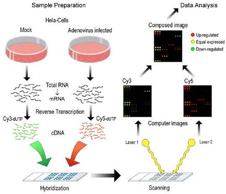
(image used with permission of Fredrik Granberg)
The two labelled samples are allowed to hybridize to the probes on the array. In theory, there are sufficient excess probes so that hybridization is not competitive. As a result, it is possible to obtain estimates of the quantity of the matching nucleotide from each sample.
For each channel, intensity is recorded for each pixel and then summarized into foreground and background measures for each probe.
The two-channel design was originally formulated to compensate for poor printing technology. Although the spots were not uniform, both samples were subjected to the same irregularities so that a measure of relative intensity, such as log2(intensity ratio) should be quite reliable even if the individual measurements were not. Each probe on each microarray was therefore a block of size two. Although print technology has much improved, intensities of the same feature measured on a single probe are more similar than those measured on different arrays. So, we still analyze two-channel microarrays considering array to be a block of size two.
Because only two channels can be hybridized to each microarray, a number of special hybridization designs have been developed for these arrays that balance the samples that are hybridized together as well as label balance to ensure that any dye-induced biases are represented equally in all treatments. [1][2]
These days microarray print technology allows printing of multiple microarrays on the same slide. Typical slides may have 6, 12 or 24 microarrays on a single slide. Generally there is a cost saving to using slides with multiple microarrays. However, this also induces some interesting constraints. The entire slide is processed in a single batch. This means that unused microarrays are wasted. For example, if the experiment includes 72 samples, 2 samples per array, then 36 microarrays will be needed. Is it better to fully utilize 3 slides with 12 samples per slide, or 2 slides with 24 samples per slide? If the decision is to use 2 slides with 24 samples each, is it better to use 24 arrays on one slide and 12 on the other, or 18 arrays on each slide? Can the remaining 12 microarrays be used to enhance the experiment in some way, for example by including some technical replication?
Most statisticians would consider the slide to be a block. It is usually preferable to have entire replicates of the experiment in each block if possible, and not to spread replicates across blocks. So, if a complete replicate of the experiment is 6 microarrays, any of the designs discussed above are possible, and if the 24 array slides are used, it is probably best to run 3 complete replicates on each array. On the other hand, if a complete replicate of the experiment uses 18 microarrays, it is probably best to use the 24 array slides with a complete replicate on each array. As you can see, there are many variations that can be considered.
Data files for low density oligo microarrays.
Once you do the hybridization and the scanning you end up with several files. There may be a .tif file for each channel: this is the raw photograph at the wavelength of each label, with an intensity for each pixel. You also have the spot file which has the probe summary statistics such as the mean intensity, median intensity, background intensity, and so on, produced by the spot detection programs. You also have an annotation file which tells you which feature was printed at each probe location. Extended annotation files might also have the sequence and functional annotation for the feature.
Notation for Two Channel Microrrays
As mentioned earlier, the basic paradigm of the two-channel microarray is that spot to spot variability can be reduced by comparing samples hybridized to the same probe. Typically comparisons are done on the log2 scale, so that log2(ratio) are the basic unit of analysis.
Two channel microarray array data are usually reduced to two summaries for each probe M (minus)
\[\begin{align}M&=log2(R/G)\\
&= log2 R - log2 G\\
\end{align}\]
and A(average)
\[\begin{align}A&=log2(\sqrt{RG})\\
&= \frac{log2 R + log2 G}{2}\\\end{align}\]
This notation almost universal, except for the influential Churchill lab which uses I=A and R=M. This notation is less common, but is used in some papers and software.
Preprocessing of Low Density Oligo Data
There's a lot of preprocessing before we get to analysis of the features. First, there is image analysis, which is all done reliably by the imaging software. This includes the determining intensity at each pixel, and the segmentation into foreground and background for each feature. The pixel-wise information is then summarized into foreground and background expression for each feature in each channel.
On the whole, the basic summarization methods are now very reliable. Due to the quality of currently available microarrays, new entrants into the field provide high quality software for feature summarization before releasing the product for use. Most investigators using microarrays do not tinker with this preprocessing step.
Basic Quality Control
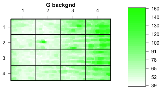
The first plot is the green background. The array is divided into rectangles that indicate how the printing was done on the old arrays - modern arrays are not segmented this way. The notable feature of this plot is the gradient of background, which is much brighter to the right. Notice from the scale that the brightest area of the background has intensity 160.
The next plot is the green foreground. It is much more uniform than the background. Notice that the intensities are mainly in the 1000's. Subtracting off the background is not going to have much effect despite the gradient.
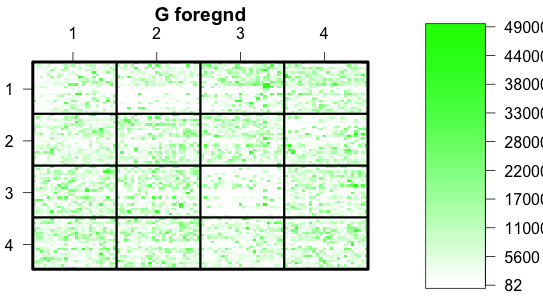
We would look at similar plots for red background and foreground. Background with magnitude similar to the foreground might indicate a poor sample. A trend in the foreground like this one seen here in the background would indicate the need for spatial normalization. This is seldom seen on modern microarrays. I would not worry too much about a trend in the background if it is orders of magnitude lower than the foreground.
We can also look at a spatial plot of M. Rectangle (3,3) looks a bit redder than the others. This will be taken care of by the normalization.
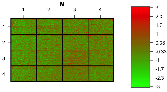
Incidentally, although I have used the Red/Green color scheme that is suggested in the documentation, it is not the best choice -- about 12 percent of men and 0.5% of women are red/green colorblind.
I do not usually do these surface plots unless I am using data from old microarrays. What I typically find most useful are a set of scatterplot matrices. Often I do these before and after normalization to check for unexpected patterns.
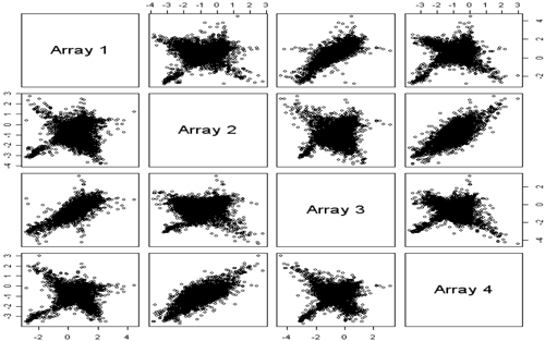
The matrices below are from a gene expression study. Genes typically have characteristic expression patterns which are fairly constant across replicates of the same treatment. As well, in most studies most of the genes are fairly constant across all treatments so that there is a strong correlation on these plots. However, M, which is a difference between expression values, should be less correlated, as the constant genes will form a circular blob around the origin.

I usually do a scatterplot matrix of the log2(intensity) for each channel. These usually look the the left plot, with a strong diagonal trend. The scatter should be tighter for replicates and somewhat looser for arrays from different treatments which may have systematic differences. A scatter of points away from the main diagonal may mean poor hybridization on an array - if the same pattern occurs on all the arrays it may be a set of control spots. The dyes do not have the same distribution of intensities, so I do not usually plot red versus green.
The A variable should also be quite similar across microarrays. The pattern often looks like the one shown above - not as nicely diagonal as the individual channels.
Finally, I plot the M variable. We expect a large cluster close to (0,0) as the biggest group of genes either do not express at all or have about the same expression level in all the samples. The irregular appearance of M in these plots suggests that normalization needs to be done.
Although I have shown scatterplots above, important aspects of the plot are difficult to assess due to number of features in each plot. To improve the visualization, we will use hexbin plots which replace the the individual points with a gray-scale that is darker where there are more data. This assists in assessing whether trends and other features of the plot are due to the bulk of the data or to a small percentage of the microarray features.
It can be difficult to determine the probe intensity distribution from the scatterplots so boxplots are often done. Each boxplot represents an entire array. If physical normalization was done we expect the median of the boxes to be about the same for red, green and A (all on the log2 scale) and for the median of the M boxes to be very close to zero. The fact that the medians are all below zero in the plot below probably means that the scanner settings for the two wavelengths were not comparable - not that the samples labelled with Cy3 had higher expression. The microarrays below need to be normalized!
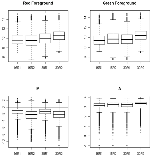
Basically my quality control strategy is to look for microarrays that have unusual features compared to the other arrays. For example, an A boxplot with unusually low spread might indicate a degraded sample. The microarrays above need normalization to equalize the mean expression in each channel on each array, (which will align the boxes) but otherwise look fine.
Dye Bias
Another assumption in two-channel microarrays is that each cDNA will bind equally to each label - i.e. a given probe will not have increased affinity for one of the dyes. The first comment on dye bias came out fairly early in 2000 or 2001 by Churchill and Kerr. They noted that a few of the probes seem to bind more strongly to one dye one that it did in the other. In fact, some of the reagent vendors include dye biased spike-ins as part of their routine quality control.
Churchill and Kerr therefore proposed a number of experimental designs for 2-channel microarrays that ensured that each sample was labelled and hybridized twice - once with Cy3 and once with Cy5. Statistical considerations show that it is not necessary to use technical replicates for this purpose - it is more effective to label biological replicates in a so-called "dye-swap" or "dye-balanced" design, so that biases balance out.
Shortly after the Churchill and Kerr reports, researchers were reporting 30% to 40% on the probes had dye bias. However, this proved to be due to degradation of Cy5 due to atmospheric conditions. In particular, Cy5 degrades rapidly in the presence of ozone which is a common pollutant (which is often high in central Pennsylvania). Again this is not a problem with modern processing, as the arrays are processed and stored in controlled environmental conditions.
The scatterplot matrix below shows what M looks like when you find dye bias due to dye degradation. If this occurs with microarrays you are using, you should complain to your microarray core facility. If you are using historical microarrays for planning or comparison purposes, my suggestion is that you NOT use a dataset showing this type of pattern. The intensities will not be reliable and there is no way to fix the samples.
Normalization
Some type of normalization is almost always done to remove array-specific artifacts. "Normalization" does not refer to the Normal distribution, but is used in the sense of equalizing measurements across samples to attempt to achieve the ideal situation that identical samples would provide identical measurements. At best, normalization is an approximation to this ideal, and the methods require some assumptions that may be violated in some types of experiments.
1. In many experiments the nucleotide samples are put through a bioanalyzer to measure the total concentration of nucleotides. The samples are often manipulated manually to physically normalize them to the same concentration. This is based on an assumption that the amount of nucleotides produced by the tissues should not vary by tissue or by treatment. When this is not the case - for example if one of the treatment shuts down or revs up gene expression or if some treatments induce genome duplications - then physical normalization can remove the most important treatment effects. Special techniques will be needed for experiments in which the "equal quantities of nucleotides in all samples" assumption is incorrect. The normalization methods discussed here, including methods using spiked in controls, are best suited when the assumption is correct.
2. The second assumption is that the probes are arranged randomly on the microarray surface so that any local high or low hybridization regions should be due to technical artifacts. When the probes are not arranged randomly, high and low regions may be due to biological effects. In this case, spatial normalization of the microarray, which attempts to remove spatial artifacts, will incorrectly "flatten" the signal.
3. The third basic (and extremely important) assumption is that the treatment effects are equally likely to induce up- or down- regulation of the genes in any pair of of treatments. This is more important than the often cited assumption that most genes do not differentially express.
The first normalization step is usually background correction. The basic assumption is that the foreground intensities should be observed as additional signal on top of the background. The simplest background correction is simply to subtract the background from the foreground - a disadvantage of this method is the possibility of computing negative foreground intensities, which would appear to indicate feature quantities below zero. Other methods for background correction include subtracting a percentage of the background chosen so that all foreground intensities are non-negative, or more complicated modeling based on the distribution of the background signal. We are going to use standard methods which are the software defaults.
The next step in normalization uses the assumption that there are aspects of the microarrays that should be the same on all the arrays in the study. It may be the median or mean intensity and SD of all the probes, the median intensity of a set of known probes (often call "house-keeping" genes) or a set of artificial probes printed for the purpose of normalization (control probes) with complementary synthesized complements added ("spiked in") to the samples at known intensities.
4. M should be independent of A.
This assumption means that if we plot M versus A, there should not be any type of trend.
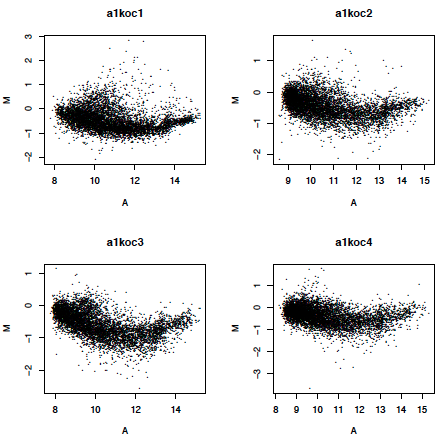
Below is a plot of M versus A for some microarrays in a study of a knock-out mouse (ApoAI) versus wildtype. Note the curvature in the plot which violates the assumption of independence of M and A. While there are many possible reasons for such a trend, I have seen someone induce various trends using a single microarray, just by adjusting the scanner settings. Usually we assume that the trend is a scanner artifact and use statistical normalization to flatten out the plot.
Lo(w)ess Normalization
Loess normalization is based on the loess method for estimating a smooth (possibly nonlinear) trend. It works by using a sliding window, and fitting the linear regression of Y on X (or in this case of M on A) in the window. The predicted value at the center of the window is the estimated value of the smooth curve. A demo can be found by clicking here. If you want to try this yourself, you can download ApoAI.RData from ANGEL, and install the R package TeachingDemos. Then follow the instructions in the demo. It will be easier to view the demo if you click on full screen mode.
A similar smoothing method called lowess is sometimes used instead of loess. The main difference between the methods is that loess uses least squares regression which is not robust to outliers, while lowess uses a method less affected by outliers.
Loess normalization estimates the trend curve on the plot of M versus A and then computes the deviations of each M-value from value expected on the curve - i.e. the residuals. The deviations are considered to be the normalized data, which enforces assumptions 3 and 4. The mean deviation is 0, which is why assumption 1 is important.
On some MA plots you will see diagonal or "V" shaped lines. These are due to truncation at detection limit (at the low end, presumably for non-expressing features) and saturation (at the high end, either due to poor scanner settings or samples that are too concentrated). As long as only a few features are in the lines, this should not affect your analysis too strongly.
Spatial Loess is can be used with there is spatial variation on the array surface, such as seen on the green background above. Instead of smoothing M versus A, the first step is smoothing R and G (separately) against the spatial coordinates to remove spatial effects. Then the usual MA loess is done. However, due to better printing and processing this is seldom necessary with modern gene expression microarrays.
Loess normalization "works" when genes are equally likely to over or under-express. It will "kill" your results if you have preferential up or down regulation in a lot of genes. It is assuming that across all levels of expression, and most genes up and down regulation are equally likely. If this is not true then Loess normalization is not the right thing to do and you will have to find other ways to normalize.
One problem I see frequently is that investigators use the default settings for programs such as normalization without thinking through the implications. The bottom line is that there's nothing automatic about data analysis of any sort!
Notice that Loess normalization is a "within array" normalization. Each two-channel microarray is normalized separately. This forces the MA curve to be flattened on each array, but does not equalize other features of the data.
Other Normalizations
There are many other types of normalizations in the literature.
Other Within Array Normalizations
Within Array Centering involves taking the mean or median of all the expressions and subtracting them from all the expression values. This forces all of the arrays to have a mean or median of zero without changing the variance of the genes. It enforces assumption 1.
Spike-in Normalization One thing that you can do if you expect different preferential differential expression either up or down is to use spiked in controls. These are either artificially synthesized DNA or cDNA from a distant species which will not match any of the species-specific probes on the microarray. Matching probes are then printed on the array. This foreign DNA is then added to each sample in known amounts which should be the same in every sample. To help with normalization, it is useful to have several different spiked in controls which can be added in different concentrations. The loess curve can then be built with just the spike-ins. This is a particularly useful method if you expect to violate assumptions 1, 3 or 4.
Housekeeping gene normalization: Housekeeping genes are supposed to be genes that express the same under all the different conditions that you're interested in. There is software that will search for housekeeping genes and then tries to normalize the array based on making the level of these genes equal. There are a number of biological concerns about whether there really are housekeeping genes that can be used for this purpose. One clever idea is to print special probes that are a mix of probes from the putative housekeeping genes. Expression levels on these mixed probes will be an average of levels on all the components, and so should be more similar across treatments than any one gene.
Removal of Unwanted Variation (RUV): This is a method that is somewhat similar to the use of housekeeping genes. A set of genes that are assumed not to differentially express in the experiment is used and covariation of these genes across the entire experiment is estimated using principal components analysis (PCA), a method for finding a weighted average of the genes that best represents the variability among the samples. Since these genes are not supposed to differentially express, it is assumed that variability due to systematic technical differences among the arrays. A small number of components (often 1- 3) are selected using standard PCA methods. These components are used as covariates during the differential expression analysis. Because the large set of nondifferentially expressing genes is reduced to a summary of the main trends, this method should be more robust than the housekeeping gene method if some of the selected genes actually do differentially express.
Between Array Normalizations
Although within microarray normalization often works well for two-channel microarrays, it does not enforce assumption 1 and it cannot be used with single channel arrays. A number of methods are used to normalize between microarrays.
Scale Normalization: After using loess normalization to remove association of M with A and enforce the same mean (or median) on every array, a simple across array normalization is to rescaled (within each microarray) so that each microarray has either the same SD across genes or the same interquartile range. The idea is that differences in spread may be due to technical issues, but that the relative spreads should be the same in every microarray. Once scale normalization is done, the boxplots of the microarrays look very uniform.
Quantile Normalization: Quantile Normalization is a very severe method that forces the distribution of intensities for the probes to be the same in every microarray. The idea is simple: for each microarray, rank the intensity values from smallest to largest (ignoring the probe id). Take the lowest intensity from each microarray and take the median of these values. Replace the lowest intensity by this median. Then repeat for the 2nd lowest, 3rd lowest, etc. When the method is complete, the set of intensity values on every microarray is identical, although the values are attached to different probes on different microarrays.
Quantile normalization can erase real differences among treatments. However, it is widely used as part of other normalizations. For example, "single channel normalization of two-channel arrays" first does loess normalization of M, then uses quantile normalization of A (so that the probe totals are the same on every microarray) and then reconstructs log2(R) and log2(G) from the normalized M and A (see below). Another use for quantile normalization is on microarrays that have multiple probes per gene. Quantile normalization is used on the probes before they are summarized into gene-wise summaries.
Separate Channel Normalization of Two Channel Arrays: Separate channel normalization of two channel arrays produces a better analysis than analysis of M, especially for complicated experimental designs.
If you remember, \(M = log2(R) - log2(G)\) and \(A = 1/2 )log2(R) + log2(G))\). To convert back:
\(log2(R)=A+M/2\)
\(log2(G)=A-M/2\)
Separate channel normalization is a between-array method that starts with loess normalization of M (within array), quantile normalization of A (between arrays) and then reconstruction of log2(R) and log2(G) from the normalized values of M and A.

