4.4 - Estimating \(m_0\) (or \(\pi_0\))
The proportion of hypotheses that are truly null is an important parameter in many situations. For example, when comparing normal and diseased tissues we might hypothesize a greater number of genes have changed response in the normal tissue than in the diseased when challenged by a toxin.
For multiple testing adjustments, the proportion of null hypotheses among the m tests is important, because we need only adjust for the \(m_0=\pi_0 m\) tests which are actually null. The other \(m-m_0\) can contribute only to the true discoveries.
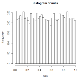
Estimation of \(\pi_0\) starts with the observation that when the test statistic is continuous, then the distribution of p-values for the null tests is uniform on the interval (0,1). This is because for any significance level \(\alpha\) the proportion of tests with p-value less than \(\alpha\) is \(\alpha\). By subtraction, we can see that the proportion of tests in any interval inside (0,1) is just the length of the interval.
Below we see a histogram of p-values from t-tests on data simulated to be 10000 2-sample tests. For each 2-sample test, both samples have the same mean and SD. Since the means are the same, the null hypothesis is true. We can see the distribution is not quite uniform, but is pretty close because these are "observed" values and so have deviations from the ideal histogram. Below this histogram is a histogram in which the two samples have different means but the same power to detect the difference. As expected, the p-values are skewed to small values. The percentage of p-values in this histogram with p-value less than \(\alpha\) is the power of the test when significance is declared at level \(\alpha\).
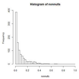
Notice that in the histogram of non-null p-values, there are very few p-values bigger than 0.2 and almost none bigger than 0.5.
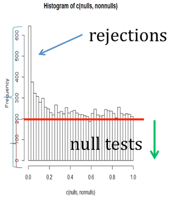
Of course when we actually test many features, some of which have the same means in both samples and some of which do not, we get a mix of histograms of this type. We should get a histogram something like the one below. In each bin of the histogram, we do not know which tests come from the truly null hypotheses, and which from the truly non-null. But we do know that the large p-values come mostly from the null distribution, and that the histogram should be fairly flat where most of the p-values come from the null. The red line shows an estimate of what the part of the histogram coming from the null should look like (although it might be a bit lower than it should be, comparing with the top histogram above).
There are several estimators of \(\pi_0\) based on this picture. Some try to estimate where the histogram flattens out. The two simplest are Storey's method and the Pounds and Cheng method.
The Pounds and Cheng [1] method is based on noting that the expected average of the null p-values is 0.5. They then assume that all of the non-null p-values are exactly 0. Then \(\hat{\pi}_0=2*\text{average}(\text{p-value})\) because on average we expect the average p-value to be \(\pi_0*0.5+(1-\pi_0)*0)\).
Storey’s method [2] uses the histogram directly, assuming that all p-values bigger than some cut-off \(\lambda\) come from the null distribution. Then we expect \(m_0(1-\lambda)\) of the tests to have p-value greater than \(\lambda\). We then count and get some number \(m_\lambda\) p-values in this region, giving us \(\hat{m}_0=m_\lambda /(1- \lambda)\) or \(\hat{\pi}_0 = m_\lambda / (m*(1-\lambda)) \) . Sophisticated implementations of the method estimate a value for \(\lambda\) but \(\lambda=0.5\) works quite well in most cases.
[1] Storey, John D. "A direct approach to false discovery rates." Journal of the Royal Statistical Society: Series B (Statistical Methodology) 64.3 (2002): 479-498.https://www.genomine.org/papers/directfdr.pdf
[2] Pounds, Stan, and Cheng Cheng. "Improving false discovery rate estimation."Bioinformatics 20.11 (2004): 1737-1745. https://bioinformatics.oxfordjournals.org/content/20/11/1737.full.pdf

