Printer-friendly version

Example 1

To make things simple in this example we work with a training dataset of one dimensional data. Our training data set contains six data points as follows:

Training set: {1.2, 5.6, 3.7, 0.6, 0.1, 2.6}.

Here we want to apply the k-means algorithm to get 2 prototypes, or centroids, \({z_1, z_2}\).

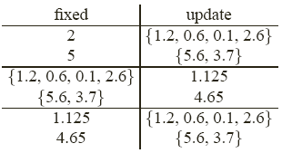
Initialization: I will start by randomly picking \(z_1 = 2\) for the first prototype, \(z_2 = 5\) for the second prototype. Let's see how k-means works ...

In the first step, we have the two prototypes initialized to 2 and 5. Now, with these two prototypes, a nearest neighbor partition of the sample points is performed. For every one of the six points, I compute its distance to 2 and 5, and find whichever is closer and assign the data point to that prototype. For instance, 1.2, 0.6, 0.1 and 2.6 are closer to 2 than to 5. Therefore, they are put together in the first group corresponding to the first prototype. The other data points, 5.6 and 3.7, are closer to 5 than to 2. They are put into the second prototype. The table below records our progress:

In the next step, I fix the partition. This means the grouping of the points will not be changed, however, we will compute the mean of the first group and the mean of the second group. We can see that the mean is not guaranteed to be the same as the values we started with. For the first group, the mean is 1.125, and for the second group, the mean is 4.65

Next, I repeat the iteration. We fix the two prototypes 1.125 and 4.65, then update the partition by the nearest neighbor rule. We will check every point to see whether it is closer to the first prototype or the second. This determines whether it goes into the first group or the second.

We find that the same four values are closer to 1.125 and the other two values are closer to 4.65. Here we can see that the assignment from the previous iteration is identical to the one just computed. This means that we no longer need to continue the iteration because if we do it again, we will get the same result for the prototypes.  The algorithm already converged.

The final result is that the two prototypes are: \(z_1 = 1.125\), \(z_2 = 4.65\). The objective function (the Euclidean distance squared added over all the points) is \(L(Z, A) = 5.3125\).

Example 2

Next, we show that starting from a different initialization, k-means can lead to a different result.

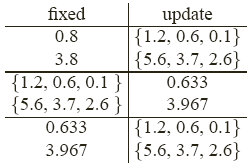
This time let's say we randomly pick \(z_1 = 0.8\), \(z_2 = 3.8\) as our prototypes and we go through the same procedure. This time the table shows us that the data was divided into two groups. 1.2, 0.6, and 0.1 are closer to 0.8; and 5.6, 3.7, and 2.6 closer to 3.8. Then we compute the mean for each group. This results in 0.633 for the first group and 3.967 for the second group as shown below.

When the assignment function from the previous iteration is identical to the one just computed, we can stop. The final result this time is: \(z_1 = 0.633\), \(z_2 = 3.967\). The objective function is \(L(Z, A) = 5.2133\). The objective function value obtained in Example 1 was 5.3125.  Therefore, this second result is better.

It can be shown that \({z_1 = 0.633, z_2 = 3.967}\) is the global optimal solution for this example. Unfortunately, however, until we get the results, there is no way to know at the beginning which initialization is going to be better. In practice, we do not have an efficient way to find the global optimal.