1(a) .4 - Terminology
Notation
Input X: X is often multidimensional.
Each dimension of X is denoted by Xj and is referred to as a feature or an independent (predictor) variable or simply, variable, (depending on what area of study you are from).
Output Y : called the response or dependent variable.
Response is available only when learning is superviused.
The Nature of Data Sets
Quantitative: Measurements or counts, recorded as numerical values, e.g. Height, Temperature, # of Red M&M’s in a bag
Qualitative: Group or categories
Ordinal: possesses a natural ordering, e.g. Shirt sizes (S, M, L, XL)
Nominal: just name of the categories, e.g. Marital Status, Gender, Color of M&M’s in a bag
Self-check
Identify the response and the predictor variables as well as the variable type.
Think About It!
Come up with an answer to these questions by yourself and then click the icon on the left to reveal the answer.
1. Does a person’s hometown influence the amount they would pay for a single CD?
2. Do men with higher education levels have higher income?
3. Is there a relationship between gender and favorite kind of music?
|
Supervised Learning versus Unsupervised Learning If Y is available in the training data, then learning method is supervised. If Y is unavailable (or ignored even if available), then the method is unsupervised. |
Supervised Learning is essentially of two types:
- Regression: the response Y is quantitative.
- Classification: the response is qualitative, or categorical.
|
Regression (Quantitative) versus Classification (Qualitative)
G ∈ G = {1, 2, ... , K}. – If Y is quantitative, then the learning algorithm is a regression problem. If Y is qualitative, the learning algorithm is a classification problem |
Ideally a learning algorithm will have the following properties
- The algorithm will be a good fit to the data. Since the model is developed using the training data, the model is expected to fit the training data well.
- The algorithm will be as robust as possible. A robust algorithm is expected to do well in case of test data; i.e. the algorithm will have high predictive power.
A 'good' predictive model developed using the training data must also work well on the test data. This may seem to be true by default, but it is not! While fitting the training data the model should not be too close to the data because, in the future, when new data is obtained there is no guarantee that they will be an exact replica of the training data. Hence is the need for the model to be robust.
A simpler model, therefore, tends to be more robust compared to a complex one, in the sense that it may have high predictive power. A complex model may follow the pattern in the training data too closely and hence its performance in the test data may be worse. On the other hand, a simple model does not fit the training data aggressively. Hence there is always a trade-off which is manifested through the following equivalent concepts.
- Training error versusTest error
- Bias versus Variance
Bias is a measure of how closely a model resembles reality. If a linear model is proposed when the true relationship between X and Y is quadratic, the proposed model is biased. If the same learning algorithm is applied to multiple independent training data, a different predictor estimate will result. If the average of these predictors is the same as the true value of the statistic in consideration, then the prediction is unbiased. Bias tends to be smaller when a model includes more parameters and complex relationship. Complex models have 'tuning knobs' to fine tune the model, but it is harder to find the right position for more 'knobs'. Bias is the systematic part of the difference between model and truth. Variance, on the other hand, is a measure of how much the predictor estimate differs when different training data is used. Variance tends to be higher for more complex models. Finding a balance between bias and variance is the objective of developing an optimum predictive model because the accuracy of a model is affected by both.
Training error reflects whether the data fits well. Testing error reflects whether the predictor actually works on new data. A model with the smallest training error will not necessarily provide the smallest test error.
- Fitting versus Overfitting
- Empirical Risk vs. Model Complexity
An overfitted model follws the training data too closely. It may have low bias but its variance will be high. This indicates that the predictor works very well on the training data but it performs substantially worse on the test data.
Empirical risk is the error rate based on the training data. If the model is more complex, then it tends to yield a smaller empirical risk but at the same time it is less robust, i.e., has higher variance. Some classification method, such as support vector machine, directly trade off empirical risk and model complexity.
Note that all of the above concepts summarizes one single concept --- A learning algorithm has to strike a perfect balance between being complex and robust so that it performs the best possible way in the training as well as in the test sample.
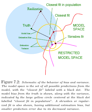
Below is a very interesting figure from "The Elements of Statistical Learning" which tries to explain the above ideas. Note that the static diagram is attempting to capture something that is very dynamic.
 The Truth at the center of the blue circle is what the data mining process tries to get at. Unfortunately the truth is not revealed to the practitioner! What is given is a sample data set which has an empirical distribution, possibly contained anywhere in the blue circle.
A large (more complex) model space is compared with a smaller one (more restricted). The two yellow circles indicate the range of the estimated models obtained under the two model spaces. Consider the larger model space, the average model obtained is indicated by the center of the large yellow circle. The difference between this center and the truth is the bias for the larger model space. Similarly, the difference between the truth and the center of the smaller yellow circle is the bias for the smaller model space. The smaller model space has larger bias. On the other hand, the resulting model from the smaller space does not vary as much as that from the larger space, that is, the variance is smaller.
Although the larger model space is in average better (smaller bias), the particular model is more likely to be poor because the variation from the average is high.
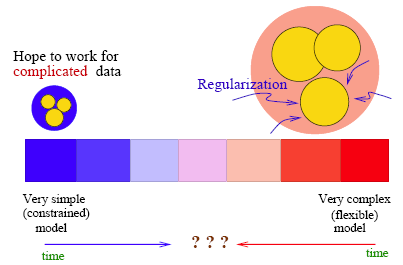
The Learning Spectrum
From a historical perspective there are two ends of the spectrum regarding learning or classification. At one end lie simple models that are very constrained. On the other end, there are very complex models that could be extremely flexible. Over the years research activities have been pushing forward a compromise or balance between model complexity and flexibility. Regularization is added to the complex models on one side, and model extension is made to the simple models on the other. Striking the perfect balance is the name of the game!


