1(a) .5 - Classification Problems in Real Life
Here are a few interesting examples to illustrate the widespread application of prediction algorithms.
1 - Email Spam
The goal is to predict whether an email is a spam and should be delivered to the Junk folder.
There are more than one method of identifying a mail as a spam. A simple method is discussed.
The raw data comprises only the text part but ignores all images. Text is a simple sequence of words which is the input (X). Goal is to predict the binary response Y: spam or not.
First step is to process the raw data into a vector, which can be done in several ways. The method followed here is based on the relative frequencies of most common words and punctuation marks in e-mail messages. A set of 57 such words and punctuation marks are pre-selected by researchers. This is where domain knowledge plays an important role.
Given these 57 most commonly occurring words and punctuation marks, then, in every e-mail message we would compute a relative frequency for each word, i.e., the percentage of times this word appears with respect to the total number of words in the email message.
In the current example 4601 e-mail messages were considered in the training sample. These e-mail messages were identified as either a good e-mail or spam after reading the mails and assuming implicitly that human decision is perfect (an arguable point!). Relative frequency of the 57 most commonly used words and punctuation based on this set of mails was constructed. This is an example of supervised learning as in the training data the response Y is known.
In future when a new e-mail message is received, the algorithm will analyze the text sequence and compute the relative frequency for these 57 identified words. This is the new input vector to be classified into spam or not through the learning algorithm.
2 - Handwritten Digit Recognition
Goal is to identify images of single digits 0 - 9 correctly.
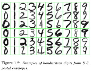
The raw data comprises images that are scaled segments from five digit ZIP codes. In the diagram below every green box is one image. The original images are very small, containing only 16 × 16 pixels. For convenience the images below are enlarged, hence the pixelation or 'boxiness' of the numbers.

Every image is to be identified as 0 or 1 or 2 ... or 9. Since the numbers are handwritten, the task is not trivial. For instance, a '5' sometimes can very much look like a '6', and '7' is sometimes confused with '1'.
To the computer, an image is a matrix, and every pixel in the image corresponds to one entry in the matrix. Every entry is an integer ranging from a pixel intensity of 0 (black) to 255 (white). Hence the raw data can be submitted to the computer directly without any feature extraction. The image matrix was scanned row by row and then arranged into a large 256 dimensional vector. This is used as the input to train the classifier.Note that this is also a supervised learning algorithm where Y, the response, is multi-level and can take 10 values.
3 - Image segmentation:
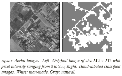
Here is a more complex example of image processing problem. The satellite images are to be identified into man-made or natural regions. For instance in the aerial images shown below, buildings are labeled as man-made, and the vegetation areas are labeled as natural.
These grayscale images are much larger than the previous example. These images are 512 × 512 pixels and again, because these are grayscale images we can present pixel intensity with numbers 0 to 255.

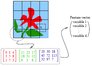
In the previous example of hand-written image identification, because of small size of the images, no feature extraction was done. However in this problem feature extraction is necessary. A standard method of feature extraction in an image processing problem is to divide images into blocks of pixels, or to form a neighborhood around each pixel. As is shown in the following diagram, after dividing the images into blocks of pixels or forming a neighborhood around each pixel, each block may be described by several features. As we have seen in the previous example, grayscale images can be represented by one matrix. Every entry in a greyscale image is an integer ranging from a pixel intensity of 0 (black) to 255 (white). Color images are represented by values of RGB (red, green and blue). Color images therefore are represented by 3 such matrices as seen below.

For each block, a few features (or statistics) may be computed using the color vectors for the pixels in the block. This set forms a feature vector for every block.
Examples of features:
- Average of R, G and B values for pixels in one block
- Variance of the brightness of the pixels (brightness is the average of RGB color values). Small variance indicates the block is visually smooth.
The feature vectors for the blocks sometimes are treated as independent samples from an unknown distribution. Ignoring f the spatial dependence among feature vectors results in performance loss. To make the learning algorithm efficient the spatial dependence needs to be exploited. Only then the accuracy in classification will improve.
4 - Speech Recognition
Another interesting example of data mining deals with speech recognition. For instance, if you call the University Park Airport, the system might ask you your flight number, or your origin and destination cities. The system does a very good job recognizing city names. This is a classification problem, in which each city name is a class. The number of classes is very big, but finite.

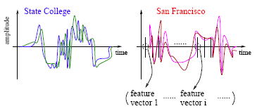
The raw data involves voice amplitude sampled at discrete time points (a time sequence), which may be represented in the waveforms as shown above. In speech recognition, a very popular method is the Hidden Markov Model.
At every time point, one or more features, such as frequencies, are computed. The speech signal essentially becomes a sequence of frequency vectors. This sequence is assumed to be an instance of a hidden Markov model (HMM). An HMM can be estimated using multiple sample sequences under the same class (e.g., city name).
Hidden Markov Model (HMM) Methodology:
HMM captures the time dependence of the feature vectors. The HMM has unspecified parameters that need to be estimated. Based on the sample sequences, model estimation takes place and a HMM is obtained. This HMM is like a mathematical signature for each word. Each city name, for example, will have a different signature. In the diagram above the signatures corresponding to State College and San Francisco are compared. It is possible that several models are constructed for one word or phrase. For instance, there may be a model for a female voice as opposed to another for a male voice.
When a customer calls in for information and utters origin or destination city pairs, the system computes the likelihood of what the customer uttered under possibly thousands of models. The system finds the HMM that yields the maximum likelihood and identifies the word as the one associated with that HMM.
5 - DNA Expression Microarray
Our goal here is to identify disease or tissue types based on the gene expression levels.
For each sample taken from a tissue of a particular disease type, the expression levels of a very large collection of genes are measured. The input data goes through a data cleaning process. Data cleaning may include, but is certainly not limited to, normalization, elimination of noise and perhaps log-scale transformations. Large volume of literature exists on the topic of cleaning microarray data.
In the example considered 96 samples were taken from 9 classes or types of tissues. It was expensive to collect the tissue samples, at least in the early days. Therefore, the sample size is often small but the dimensionality of data is very high. Every sample is measured on 4026 genes. very often microarray data analysis has its own challenges with small number of observations and very large umber of features from each observation.
6 - DNA Sequence Classification
Each genome is made up of DNA sequences and each DNA segment has specific biological functions. However there are DNA segments which are non-coding, i.e. they do not have any biological function (or their functionalities are not yet known). One problem in DNA sequencing is to label the sampled segments as coding or non-coding (with biological function or without).
The raw DNA data comprises sequences of letters, e.g., A, C, G, T for each of the DNA sequences. One method of classification assumes the sequences to be realizations of random processes. Different random processes are assumed for different classes of sequences.
In the above examples on classification several simple and complex real-life problems are considered. Classification problems are faced in a wide range of research areas. The raw data can come in all sizes, shapes and varieties. A critical step in data mining is to formulate a mathematical problem from a real problem. In this course the focus is on the learning algorithms. The formulation step is largely left out.

