5.4 - The Lasso
Lasso
A ridge solution can be hard to interpret because it is not sparse (no \(\beta\)'s are set exactly to 0). What if we constrain the $L1$ norm instead of the Euclidean ($L2$) norm?
\begin{equation*}
\textrm{Ridge subject to:} \sum_{j=1}^p (\beta_j)^2 < c.
\end{equation*}
\begin{equation*}
\textrm{Lasso subject to:} \sum_{j=1}^p |\beta_j| < c.
\end{equation*}
This is a subtle, but important change. Some of the coefficients may be shrunk exactly to zero.
The least absolute shrinkage and selection operator, or lasso, as described in Tibshirani (1996) is a technique that has received a great deal of interest.
As with ridge regression we assume the covariates are standardized. Lasso estimates of the coefficients (Tibshirani, 1996) achieve $\min_\beta (Y-X\beta)'(Y-X\beta) + \lambda \sum_{j=1}^p|\beta_j|$, so that the L2 penalty of ridge regression \(\sum_{j=1}^{p}\beta_{j}^{2}\) is replaced by an L1 penalty, \(\sum_{j=1}^{p}|\beta_{j}|\).
Let $c_0 = \sum_{j=1}^p|\hat{\beta}_{LS,j}|$ denote the absolute size of the least squares estimates. Values of $0< c < c_0$ cause shrinkage towards zero.
If, for example, $c = c_0/2$ the average shrinkage of the least squares coefficients is 50%. If $\lambda$ is sufficiently large, some of the coefficients are driven to zero, leading to a sparse model.
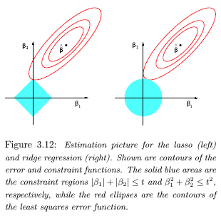
Geometric Interpretation
The lasso performs $L1$ shrinkage, so that there are "corners'' in the constraint, which in two dimensions corresponds to a diamond. If the sum of squares "hits'' one of these corners, then the coefficient corresponding to the axis is shrunk to zero.
![]()
As $p$ increases, the multidimensional diamond has an increasing number of corners, and so it is highly likely that some coefficients will be set equal to zero. Hence, the lasso performs shrinkage and (effectively) subset selection.
In contrast with subset selection, Lasso performs a soft thresholding: as the smoothing parameter is varied, the sample path of the estimates moves continuously to zero.
Least Angle Regression
The lasso loss function is no longer quadratic, but is still convex:
\begin{equation*}
\textrm{Minimize:} \sum_{i=1}^n(Y_i-\sum_{j=1}^p X_{ij}\beta_j)^2 + \lambda \sum_{j=1}^p|\beta_j|
\end{equation*}
Unlike ridge regression, there is no analytic solution for the lasso because the solution is nonlinear in $Y$. The entire path of lasso estimates for all values of $\lambda$ can be efficiently computed through a modification of the Least Angle Regression (LARS) algorithm (Efron et al. 2003).
Lasso and ridge regression both put penalties on $\beta$. More generally, penalties of the form $\lambda \sum_{j=1}^p |\beta_j|^q$ may be considered, for $q\geq0$. Ridge regression and the lasso correspond to $q = 2$ and $q = 1$, respectively. When $X_j$ is weakly related with $Y$, the lasso pulls $\beta_j$ to zero faster than ridge regression.
Inference for Lasso Estimation
The ordinary lasso does not address the uncertainty of parameter estimation; standard errors for $\beta$'s are not immediately available.
For inference using the lasso estimator, various standard error estimators have been proposed:
-
Tibshirani (1996) suggested the bootstrap (Efron, 1979) for the estimation of standard errors and derived an approximate closed form estimate.
-
Fan and Li (2001) derived the sandwich formula in the likelihood setting as an estimator for the covariance of the estimates.
However, the above approximate covariance matrices give an estimated variance of $0$ for predictors with $\hat{\beta}_j=0$. The "Bayesian lasso" of Park and Casella (2008) provides valid standard errors for $\beta$ and provides more stable point estimates by using the posterior median. The lasso estimate is equivalent to the mode of the posterior distribution under a normal likelihood and an independent Laplace (double exponential) prior:
\begin{equation*}
\pi(\beta) = \frac{\lambda}{2} \exp(-\lambda |\beta_j|)
\end{equation*}
The Bayesian lasso estimates (posterior medians) appear to be a compromise between the ordinary lasso and ridge regression. Park and Casella (2008) showed that the posterior density was unimodal based on a conditional Laplace prior, $\lambda|\sigma$, a noninformative marginal prior $\pi(\sigma^2) \propto 1/\sigma^2$, and the availability of a Gibbs algorithm for sampling the posterior distribution.
\begin{equation*}
\pi(\beta|\sigma^2) = \prod_{j=1}^p \frac{\lambda}{2\sqrt{\sigma^2}}\exp(-\frac{\lambda |\beta_j|}{2\sqrt{\sigma^2}})
\end{equation*}
Compare Ridge Regression and Lasso
The colored lines are the paths of regression coefficients shrinking towards zero. If we draw a vertical line in the figure, it will give a set of regression coefficients corresponding to a fixed $\lambda$. (The x-axis actually shows the proportion of shrinkage instead of $\lambda$).
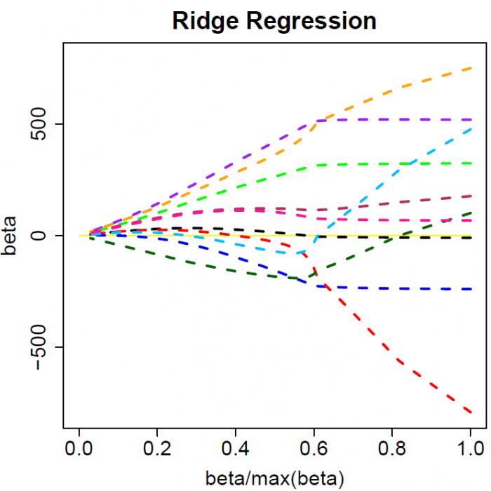
Ridge regression shrinks all regression coefficients towards zero; the lasso tends to give a set of zero regression coefficients and leads to a sparse solution.
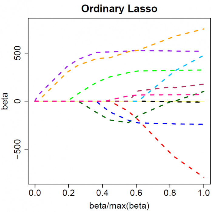
Note that for both ridge regression and the lasso the regression coefficients can move from postive to negative values as they are shrunk toward zero.
Group Lasso
In some contexts, we may wish to treat a set of regressors as a group, for example, when we have a categorical covariate with more than two levels. The grouped lasso Yuan and Lin (2007) addresses this problem by considering the simultaneous shrinkage of (pre-defined) groups of coefficients.

