Printer-friendly version

Let's illustrate why it might be beneficial in some cases to have a biased estimator. This is just an illustration with some impractical assumptions. Let's assume that \(\hat{\beta}\) follows a normal distribution with mean 1 and variance 1. This means that the true \(\beta =1\) and that the true variance when you do least squares estimation is assumed to equal 1. In practice we do not know this distribution.

Instead of \(\hat{\beta}\), we will use a shrinkage estimator for \(\beta\), \(\tilde{\beta}\), which is \(\hat{\beta}\) shrunk by a factor of a (where a is a constant greater than one). Then:

Squared loss: \(  E(\hat{\beta}-1)^2 = Var(\hat{\beta})\).

For \(\tilde{\beta} = \frac{\hat{\beta}}{a}, a \ge 1  \), \( E(\tilde{\beta}-1)^2 = Var(\tilde{\beta}) + (E(\tilde{\beta})-1)^2 = \frac{1}{a^2}+\left(\frac{1}{a}-1  \right)^2\).

Take a look at the squared difference between \(\hat{\beta}\) and the true \(\beta\) (= 1). Then compare with the new estimator, \(\tilde{\beta}\), and see how accurate it gets compared to the true value of 1. Again, we compute the squared difference between \(\tilde{\beta}\) and 1 because \(\tilde{\beta}\) itself is random and we can only talk about it in the average sense. We can think of this as a measure of accuracy - expected squared loss which turns out to be the variance of \(\tilde{\beta}\) + the squared bias.

By shrinking the estimator by a factor of a, the bias is not zero. So, it is not an unbiased estimator anymore. The variance of \(\tilde{\beta} = 1/a^2\).

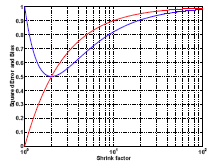
Therefore, the bigger a gets the higher the bias would be. The red curve in the plot below shows the squared bias with respect to a. When a goes to infinity, the bias approaches 1. Also, when a approaches infinity, the variance approaches zero. As you can see, one term goes up and the other term goes down. The sum of the two terms is shown by the blue curve.

You can see that the optimal is achieved at a = 2 rather than a = 1. a = 1 gives you the unbiased estimator. However, a = 2 is biased but it gives you a smaller expected loss. In this case a biased estimation may yield better prediction accuracy.

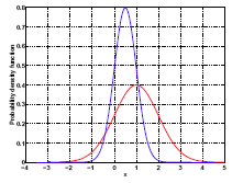
The red curve in the plot below represents the original distribution of \(\beta\) which has variance = 1. When you shrink it, dividing it by a constant greater than one, the distribution becomes more spiky. The variance is decreased because the distribution is squeezed. In the meantime, there is one negative thing going on---the mean has shifted away from 1.