Printer-friendly version

Summary Statistics

Vast amount of numbers on a large number of variables need to be properly organized to extract information from them. Broadly speaking there are two methods to summarize data: visual summarization and numerical summarization. Both have their advantages and disadvantages and applied jointly they will get the maximum information from raw data.

Summary statistics are numbers computed from the sample that present a summary of the attributes.

Measures of Location

They are single numbers representing a set of observations. Measures of location also includes measures of central tendency. Measures of central tendency can also be taken as the most representative values of the set of observations. The most common measures of location are the Mean, the Median, the Mode and the Quartiles.

Mean is the arithmatic average of all the observations. The mean equals the sum of all observations divided by the sample size.

Median is the middle-most value of the ranked set of observations so that half the observations are greater than the median and the other half is less. Median is a robust measure of central tendency.

Mode is the the most frequently occuring value in the data set. This makes more sense when attributes are not continuous.

Quartiles are division points which split data into four equal parts after rank-ordering them. Division points are called Q1 (the first quartile), Q2 (the second quartile or median), and Q3 (the third quartile). They are not necessarily four equidistance point on the range of the sample.

Similarly Deciles and Percentiles are defined as division points that divide the rank-ordered data into 10 and 100 equal segments. 

Note that the mean is very sensitive to outliers (extreme or unusual observations) whereas the median is not. The mean is affected if even a single observation is changed. The median, on the other hand, has a 50% breakdown which means that unless 50% values in a sample change, median will not change.

Measures of Spread

Measures of location is not enough to capture all aspects of  the attributes. Measures of dispersion are necessary to understand the variability of the data. The most common measure of dispersion are the Variance, the Standard Deviation, the Interquartile Range and Range.

Variance measures how far data values lie from the mean. It is defined as the average of the squared differences between the mean and the individual data values.

Standard Deviation is the square root of the variance.  It is defined as the average distance between the mean and the individual data values.

Interquartile range (IQR) is the difference between Q3 and Q1. IQR contains the middle 50% of data.

Range is the difference between the maximum and minimum values in the sample.

Measures of Skewness

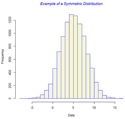
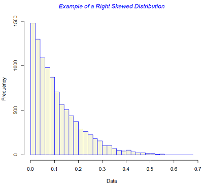
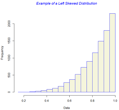
In addition to the measures of location and dispersion, the arrangement of data or the shape of the the data distribution is also of considerable interest. The most 'well-bahaved' distribution is a symmetric distribution where the mean and the median are coincident. The symmetry is lost if there exists a tail in either direction. Skewness measures whether or not a distribution has a single long tail.

Skewness is measured as:

\[ \frac{\sqrt{n} \left( \Sigma \left(x_{i} - \bar{x} \right)^{3} \right)}{\left(\Sigma \left(x_{i} - \bar{x} \right)^{2}\right)^{\frac{3}{2}}}. \]

The figure below gives examples of symmetric and skewed distributions. Note that these diagrams are generated from theoretical distributions and in practice one is likely to see only approximations.

Measures of Correlation

All the above summary statistics are applicable only for univariate data where information on a single attribute is of interest. Correlation describes the degree of the linear relationship between two attributes, X and Y.

With X taking the values x(1), … , x(n) and Y taking the values y(1), … , y(n), the sample correlation coefficient is defined as:

\[\rho (X,Y)=\frac{\sum_{i=1}^{n}\left ( x(i)-\bar{x} \right )\left ( y(i)-\bar{y} \right )}{\left( \sum_{i=1}^{n}\left ( x(i)-\bar{x} \right )^2\sum_{i=1}^{n}\left ( y(i)-\bar{y} \right )^2\right)^\frac{1}{2}}\]

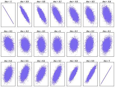
The correlation coefficient is always between -1 (perfect negative linear relationship) and +1 (perfect positive linear relationship). If the correlation coefficient is 0, then there is no linear relationship between X and Y.

In the figure below a set of representative plots are shown for various values of the population correlation coefficient ρ ranging from - 1 to + 1. At the two extreme values the relation is a perfect straight line. As the value of ρ approaches 0, the elliptical shape becomes round and then it moves again towards an elliptical shape with the principal axis in the opposite direction.