2.2 - What is the "Best Fitting Line"?
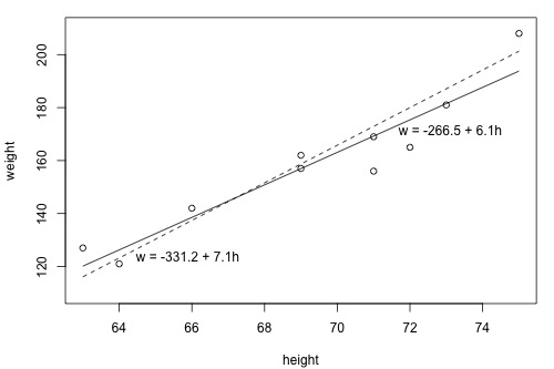
Since we are interested in summarizing the trend between two quantitative variables, the natural question arises — "what is the best fitting line?" At some point in your education, you were probably shown a scatter plot of (x, y) data and were asked to draw the "most appropriate" line through the data. Even if you weren't, you can try it now on a set of heights (x) and weights (y) of 10 students, (student_height_weight.txt). Looking at the plot below, which line — the solid line or the dashed line — do you think best summarizes the trend between height and weight?
Hold on to your answer! In order to examine which of the two lines is a better fit, we first need to introduce some common notation:
- \(y_i\) denotes the observed response for experimental unit i
- \(x_i\) denotes the predictor value for experimental unit i
- \(\hat{y}_i\) is the predicted response (or fitted value) for experimental unit i
Then, the equation for the best fitting line is:
\[\hat{y}_i=b_0+b_1x_i\]
Incidentally, recall that an "experimental unit" is the object or person on which the measurement is made. In our height and weight example, the experimental units are students.
Let's try out the notation on our example with the trend summarized by the line w = -266.53 + 6.1376 h. (Note that this line is just a more precise version of the above solid line, w = -266.5 + 6.1 h.) The first data point in the list indicates that student 1 is 63 inches tall and weighs 127 pounds. That is, x1 = 63 and y1 = 127 . Do you see this point on the plot? If we know this student's height but not his or her weight, we could use the equation of the line to predict his or her weight. We'd predict the student's weight to be -266.53 + 6.1376(63) or 120.1 pounds. That is, \(\hat{y}_1\) = 120.1. Clearly, our prediction wouldn't be perfectly correct — it has some "prediction error" (or "residual error"). In fact, the size of its prediction error is 127-120.1 or 6.9 pounds.
You might want to roll your cursor over each of the 10 data points to make sure you understand the notation used to keep track of the predictor values, the observed responses and the predicted responses:
|
As you can see, the size of the prediction error depends on the data point. If we didn't know the weight of student 5, the equation of the line would predict his or her weight to be -266.53 + 6.1376(69) or 157 pounds. The size of the prediction error here is 162-157, or 5 pounds.
In general, when we use \(\hat{y}_i=b_0+b_1x_i\) to predict the actual response yi, we make a prediction error (or residual error) of size:
\[e_i=y_i-\hat{y}_i\]
A line that fits the data "best" will be one for which the n prediction errors — one for each observed data point — are as small as possible in some overall sense. One way to achieve this goal is to invoke the "least squares criterion," which says to "minimize the sum of the squared prediction errors." That is:
- The equation of the best fitting line is: \(\hat{y}_i=b_0+b_1x_i\)
- We just need to find the values b0 and b1 that make the sum of the squared prediction errors the smallest it can be.
- That is, we need to find the values b0 and b1 that minimize:
\[Q=\sum_{i=1}^{n}(y_i-\hat{y}_i)^2\]
Here's how you might think about this quantity Q:
- The quantity \(e_i=y_i-\hat{y}_i\) is the prediction error for data point i.
- The quantity \(e_i^2=(y_i-\hat{y}_i)^2\) is the squared prediction error for data point i.
- And, the symbol \(\sum_{i=1}^{n}\) tells us to add up the squared prediction errors for all n data points.
Now, being familiar with the least squares criterion, let's take a fresh look at our plot again. In light of the least squares criterion, which line do you now think is the best fitting line?
Let's see how you did! The following two side-by-side tables illustrate the implementation of the least squares criterion for the two lines up for consideration — the dashed line and the solid line.
|
|
||||||||||||||||||||||||||||||||||||||||||||||||||||||||||||||||||||||||||||||||||||||||||||||||||||||||||||||||||||||||||||||||||||||||||||||||||||||||||||
Based on the least squares criterion, which equation best summarizes the data? The sum of the squared prediction errors is 766.5 for the dashed line, while it is only 597.4 for the solid line. Therefore, of the two lines, the solid line, w = -266.53 + 6.1376h, best summarizes the data. But, is this equation guaranteed to be the best fitting line of all of the possible lines we didn't even consider? Of course not!
If we used the above approach for finding the equation of the line that minimizes the sum of the squared prediction errors, we'd have our work cut out for us. We'd have to implement the above procedure for an infinite number of possible lines — clearly, an impossible task! Fortunately, somebody has done some dirty work for us by figuring out formulas for the intercept b0 and the slope b1 for the equation of the line that minimizes the sum of the squared prediction errors.
The formulas are determined using methods of calculus. We minimize the equation for the sum of the squared prediction errors:
\[Q=\sum_{i=1}^{n}(y_i-(b_0+b_1x_i))^2\]
(that is, take the derivative with respect to b0 and b1, set to 0, and solve for b0 and b1) and get the "least squares estimates" for b0 and b1:
\[b_0=\bar{y}-b_1\bar{x}\]
and:
\[b_1=\frac{\sum_{i=1}^{n}(x_i-\bar{x})(y_i-\bar{y})}{\sum_{i=1}^{n}(x_i-\bar{x})^2}\]
Because the formulas for b0 and b1 are derived using the least squares criterion, the resulting equation — \(\hat{y}_i=b_0+b_1x_i\)— is often referred to as the "least squares regression line," or simply the "least squares line." It is also sometimes called the "estimated regression equation." Incidentally, note that in deriving the above formulas, we made no assumptions about the data other than that they follow some sort of linear trend.
We can see from these formulas that the least squares line passes through the point \((\bar{x},\bar{y})\), since when \(x=\bar{x}\), then \(y=b_0+b_1\bar{x}=\bar{y}-b_1\bar{x}+b_1\bar{x}=\bar{y}\).
In practice, you won't really need to worry about the formulas for b0 and b1. Instead, you are are going to let statistical software, such as R or Minitab, find least squares lines for you.
One thing the estimated regression coefficients, b0 and b1, allow us to do is to predict future responses — one of the most common uses of an estimated regression line. This use is rather straightforward:
| A common use of the estimated regression line. |
\(\hat{y}_{i,wt}=-266.53+6.1376 x_{i, ht}\)
|
| Predict (mean) weight of 66"-inch tall people. |
\(\hat{y}_{i, wt}=-266.53+6.1376(66)=138.55\)
|
| Predict (mean) weight of 67"-inch tall people. |
\(\hat{y}_{i, wt}=-266.53+6.1376(67)=144.69\)
|
Now, what does b0 tell us? The answer is obvious when you evaluate the estimated regression equation at x = 0. Here, it tells us that a person who is 0 inches tall is predicted to weigh -266.53 pounds! Clearly, this prediction is nonsense. This happened because we "extrapolated" beyond the "scope of the model" (the range of the x values). It is not meaningful to have a height of 0 inches, that is, the scope of the model does not include x = 0. So, here the intercept b0 is not meaningful. In general, if the "scope of the model" includes x = 0, then b0 is the predicted mean response when x = 0. Otherwise, b0 is not meaningful. There is more discussion of this here.
And, what does b1 tell us? The answer is obvious when you subtract the predicted weight of 66"-inch tall people from the predicted weight of 67"-inch tall people. We obtain 144.69 - 138.55 = 6.14 pounds -- the value of b1. Here, it tells us that we predict the mean weight to increase by 6.14 pounds for every additional one-inch increase in height. In general, we can expect the mean response to increase or decrease by b1 units for every one unit increase in x.

