The plot of our population of data suggests that the college entrance test scores for each subpopulation have equal variance. We denote the value of this common variance as σ².

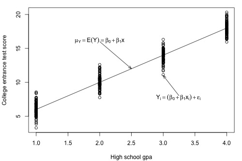
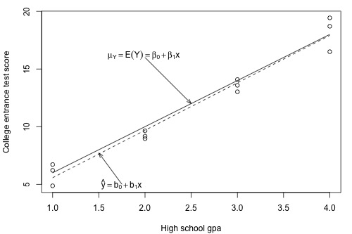
That is, σ² quantifies how much the responses (y) vary around the (unknown) mean population regression line \(\mu_Y=E(Y)=\beta_0 + \beta_1x\).

Why should we care about σ²? The answer to this question pertains to the most common use of an estimated regression line, namely predicting some future response.

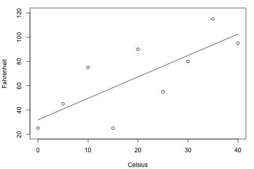
Suppose you have two brands (A and B) of thermometers, and each brand offers a Celsius thermometer and a Fahrenheit thermometer. You measure the temperature in Celsius and Fahrenheit using each brand of thermometer on ten different days. Based on the resulting data, you obtain two estimated regression lines — one for brand A and one for brand B. You plan to use the estimated regression lines to predict the temperature in Fahrenheit based on the temperature in Celsius.

Will this thermometer brand (A) yield more precise future predictions …?

… or this one (B)?

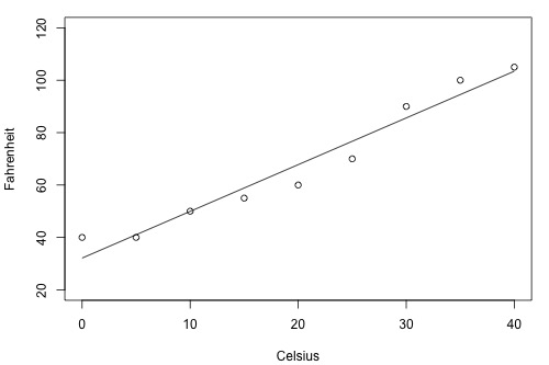
As the two plots illustrate, the Fahrenheit responses for the brand B thermometer don't deviate as far from the estimated regression equation as they do for the brand A thermometer. If we use the brand B estimated line to predict the Fahrenheit temperature, our prediction should never really be too far off from the actual observed Fahrenheit temperature. On the other hand, predictions of the Fahrenheit temperatures using the brand A thermometer can deviate quite a bit from the actual observed Fahrenheit temperature. Therefore, the brand B thermometer should yield more precise future predictions than the brand A thermometer.

To get an idea, therefore, of how precise future predictions would be, we need to know how much the responses (y) vary around the (unknown) mean population regression line \(\mu_Y=E(Y)=\beta_0 + \beta_1x\). As stated earlier, σ² quantifies this variance in the responses. Will we ever know this value σ²? No! Because σ² is a population parameter, we will rarely know its true value. The best we can do is estimate it!

To understand the formula for the estimate of σ² in the simple linear regression setting, it is helpful to recall the formula for the estimate of the variance of the responses, σ², when there is only one population.

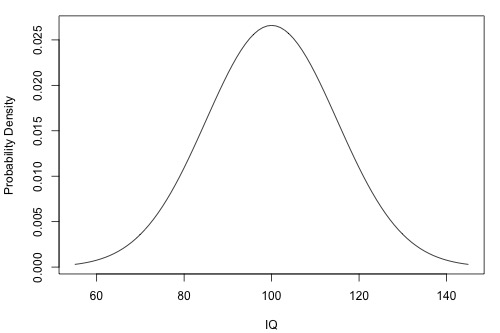
The following is a plot of a population of IQ measurements. As the plot suggests, the average of the IQ measurements in the population is 100. But, how much do the IQ measurements vary from the mean? That is, how "spread out" are the IQs?

The sample variance:

\[s^2=\frac{\sum_{i=1}^{n}(y_i-\bar{y})^2}{n-1}\]

estimates σ², the variance of the one population. The estimate is really close to being like an average. The numerator adds up how far each response y_i is from the estimated mean \(\bar{y}\) in squared units, and the denominator divides the sum by n-1, not n as you would expect for an average. What we would really like is for the numerator to add up, in squared units, how far each response y_i is from the unknown population mean μ. But, we don't know the population mean μ, so we estimate it with \(\bar{y}\). Doing so "costs us one degree of freedom". That is, we have to divide by n-1, and not n, because we estimated the unknown population mean μ.

Now let's extend this thinking to arrive at an estimate for the population variance σ² in the simple linear regression setting. Recall that we assume that σ² is the same for each of the subpopulations. For our example on college entrance test scores and grade point averages, how many subpopulations do we have?

There are four subpopulations depicted in this plot. In general, there are as many subpopulations as there are distinct x values in the population. Each subpopulation has its own mean μ_Y, which depends on x through \(\mu_Y=E(Y)=\beta_0 + \beta_1x\). And, each subpopulation mean can be estimated using the estimated regression equation \(\hat{y}_i=b_0+b_1x_i\):

The mean square error:

\[MSE=\frac{\sum_{i=1}^{n}(y_i-\hat{y}_i)^2}{n-2}\]

estimates σ², the common variance of the many subpopulations.

How does the mean square error formula differ from the sample variance formula? The similarities are more striking than the differences. The numerator again adds up, in squared units, how far each response y_i is from its estimated mean. In the regression setting, though, the estimated mean is \(\hat{y}_i\). And, the denominator divides the sum by n-2, not n-1, because in using \(\hat{y}_i\) to estimate  μ_Y, we effectively estimate two parameters — the population intercept β₀ and the population slope β₁. That is, we lose two degrees of freedom.

In practice, we will let statistical software, such as R or Minitab, calculate the mean square error (MSE) for us. For the sample of 12 high school GPAs and college test scores,

\[MSE=\frac{8.678}{12-2}=0.8678.\]

As well as displaying MSE, software typically also displays \(S=\sqrt{MSE}\), which estimates σ and is known as the regression standard error or the residual standard error. For the sample of 12 high school GPAs and college test scores, \(S=\sqrt{0.8678}=0.9315\).