Let's take a look at some examples so we can get some practice interpreting the coefficient of determination r² and the correlation coefficient r.

Example 1. How strong is the linear relationship between temperatures in Celsius and temperatures in Fahrenheit? Here's a plot of an estimated regression equation based on n = 11 data points:

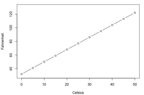
Statistical software reports that r² = 100% and r = 1.000. Both measures tell us that there is a perfect linear relationship between temperature in degrees Celsius and temperature in degrees Fahrenheit. We know that the relationship is perfect, namely that Fahreheit = 32 + 1.8 × Celsius. It should be no surprise then that r² tells us that 100% of the variation in temperatures in Fahrenheit is explained by the temperature in Celsius.

Example 2. How strong is the linear relationship between the number of stories a building has and its height? One would think that as the number of stories increases, the height would increase, but not perfectly. Some statisticians compiled data on a set of n = 60 buildings reported in the 1994 World Almanac (bldgstories.txt). Statistical software reports r² = 90.4% and r = 0.951 and produced the following plot:

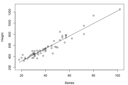
The positive sign of r tells us that the relationship is positive — as number of stories increases, height increases — as we expected. Because r is close to 1, it tells us that the linear relationship is very strong, but not perfect. The r² value tells us that 90.4% of the variation in the height of the building is explained by the number of stories in the building.

Example 3. How strong is the linear relationship between the age of a driver and the distance the driver can see? If we had to guess, we might think that the relationship is negative — as age increases, the distance decreases. A research firm (Last Resource, Inc., Bellefonte, PA) collected data on a sample of n = 30 drivers (signdist.txt). Statistical software reports that reports that r² = 64.2% and r = -0.801 and produced the following output:

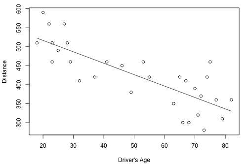
The negative sign of r tells us that the relationship is negative — as driving age increases, seeing distance decreases — as we expected. Because r is fairly close to -1, it tells us that the linear relationship is fairly strong, but not perfect. The r² value tells us that 64.2% of the variation in the seeing distance is reduced by taking into account the age of the driver.

Example 4. How strong is the linear relationship between the height of a student and his or her grade point average? Data were collected on a random sample of n = 35 students in a statistics course at Penn State University (heightgpa.txt). Statistical software reports that r² = 0.3% and r = -0.053 and produced the following output:

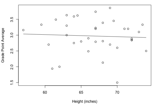
Because r is quite close to 0, it suggests — not surprisingly, I hope — that there is next to no linear relationship between height and grade point average. Indeed, the r² value tells us that only 0.3% of the variation in the grade point averages of the students in the sample can be explained by their height. In short, we would need to identify another more important variable, such as number of hours studied, if predicting a student's grade point average is important to us.