Lesson 10: Model Building
Lesson 10: Model BuildingOverview
For all of the regression analyses that we performed so far in this course, it has been obvious which of the major predictors we should include in our regression model. Unfortunately, this is typically not the case. More often than not, a researcher has a large set of candidate predictor variables from which he tries to identify the most appropriate predictors to include in his regression model.
Of course, the larger the number of candidate predictor variables, the larger the number of possible regression models. For example, if a researcher has (only) 10 candidate predictor variables, he has \(2^{10} = 1024\) possible regression models from which to choose. Clearly, some assistance would be needed in evaluating all of the possible regression models. That's where the two variable selection methods — stepwise regression and best subsets regression — come in handy.
In this lesson, we'll learn about the above two variable selection methods. Our goal throughout will be to choose a small subset of predictors from the larger set of candidate predictors so that the resulting regression model is simple yet useful. That is, as always, our resulting regression model should:
- provide a good summary of the trend in the response, and/or
- provide good predictions of the response, and/or
- provide good estimates of the slope coefficients.
Objectives
- Understand the impact of the four different models concerning their "correctness" — correctly specified, underspecified, overspecified, and correct but with extraneous predictors.
- To ensure that you understand the general idea behind stepwise regression, be able to conduct stepwise regression "by hand."
- Know the limitations of stepwise regression.
- Know the general idea behind best subsets regression.
- Know how to choose an optimal model based on the \(R^{2}\) value, the adjusted \(R^{2}\) value, MSE and the \(C_p\) criterion.
- Know the limitations of best subsets regression.
- Know the seven steps of an excellent model-building strategy.
Lesson 10 Code Files
Below is a zip file that contains all the data sets used in this lesson:
- bloodpress.txt
- cement.txt
- iqsize.txt
- martian.txt
- peru.txt
- Physical.txt
10.1 - What if the Regression Equation Contains "Wrong" Predictors?
10.1 - What if the Regression Equation Contains "Wrong" Predictors?Before we can go off and learn about the two variable selection methods, we first need to understand the consequences of a regression equation containing the "wrong" or "inappropriate" variables. Let's do that now!
There are four possible outcomes when formulating a regression model for a set of data:
- The regression model is "correctly specified."
- The regression model is "underspecified."
- The regression model contains one or more "extraneous variables."
- The regression model is "overspecified."
Let's consider the consequence of each of these outcomes on the regression model. Before we do, we need to take a brief aside to learn what it means for an estimate to have the good characteristic of being unbiased.
Unbiased estimates
An estimate is unbiased if the average of the values of the statistics determined from all possible random samples equals the parameter you're trying to estimate. That is, if you take a random sample from a population and calculate the mean of the sample, then take another random sample and calculate its mean, and take another random sample and calculate its mean, and so on — the average of the means from all of the samples that you have taken should equal the true population mean. If that happens, the sample mean is considered an unbiased estimate of the population mean \(\mu\).
An estimated regression coefficient \(b_i\) is an unbiased estimate of the population slope \(\beta_i\) if the mean of all of the possible estimates \(b_i\) equals \(\beta_i\). And, the predicted response \(\hat{y}_i\) is an unbiased estimate of \(\mu_Y\) if the mean of all of the possible predicted responses \(\hat{y}_i\) equals \(\mu_Y\).
So far, this has probably sounded pretty technical. Here's an easy way to think about it. If you hop on a scale every morning, you can't expect that the scale will be perfectly accurate every day —some days it might run a little high, and some days a little low. That you can probably live with. You certainly don't want the scale, however, to consistently report that you weigh five pounds more than you actually do — your scale would be biased upward. Nor do you want it to consistently report that you weigh five pounds less than you actually do — or..., scratch that, maybe you do — in this case, your scale would be biased downward. What you do want is for the scale to be correct on average — in this case, your scale would be unbiased. And, that's what we want!
The four possible outcomes
Outcome 1
A regression model is correctly specified if the regression equation contains all of the relevant predictors, including any necessary transformations and interaction terms. That is, there are no missing, redundant, or extraneous predictors in the model. Of course, this is the best possible outcome and the one we hope to achieve!
The good thing is that a correctly specified regression model yields unbiased regression coefficients and unbiased predictions of the response. And, the mean squared error (MSE) — which appears in some form in every hypothesis test we conduct or confidence interval we calculate — is an unbiased estimate of the error variance \(\sigma^{2}\).
Outcome 2
A regression model is underspecified if the regression equation is missing one or more important predictor variables. This situation is perhaps the worst-case scenario because an underspecified model yields biased regression coefficients and biased predictions of the response. That is, in using the model, we would consistently underestimate or overestimate the population slopes and the population means. To make already bad matters even worse, the mean square error MSE tends to overestimate \(\sigma^{2}\), thereby yielding wider confidence intervals than it should.
Let's take a look at an example of a model that is likely underspecified. It involves an analysis of the height and weight of Martians. The Martian dataset — which was obviously contrived just for the sake of this example — contains the weights (in g), heights (in cm), and amount of daily water consumption (0, 10, or 20 cups per day) of 12 Martians.
If we regress \(y = \text{ weight}\) on the predictors \(x_1 = \text{ height}\) and \(x_2 = \text{ water}\), we obtain the following estimated regression equation:
Regression Equation
\(\widehat{weight} = -1.220 + 0.28344 height + 0.11121 water\)
and the following estimate of the error variance \(\sigma^{2}\):
MSE = 0.017
If we regress \(y = \text{ weight}\) on only the one predictor \(x_1 = \text{ height}\), we obtain the following estimated regression equation:
Regression Equation
\(\widehat{weight} = -4.14 + 0.3889 height\)
and the following estimate of the error variance \(\sigma^{2}\):
MSE = 0.653
Plotting the two estimated regression equations, we obtain:
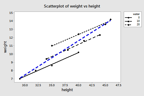
The three black lines represent the estimated regression equation when the amount of water consumption is taken into account — the first line for 0 cups per day, the second line for 10 cups per day, and the third line for 20 cups per day. The blue dashed line represents the estimated regression equation when we leave the amount of water consumed out of the regression model.
The second model — in which water is left out of the model — is likely an underspecified model. Now, what is the effect of leaving water consumption out of the regression model?
- The slope of the line (0.3889) obtained when height is the only predictor variable is much steeper than the slopes of the three parallel lines (0.28344) obtained by including the effect of water consumption, as well as height, on martian weight. That is, the slope likely overestimates the actual slope.
- The intercept of the line (-4.14) obtained when height is the only predictor variable is smaller than the intercepts of the three parallel lines (-1.220, -1.220 + 0.11121(10) = -0.108, and -1.220 + 0.11121(20) = 1.004) obtained by including the effect of water consumption, as well as height, on martian weight. That is, the intercept likely underestimates the actual intercepts.
- The estimate of the error variance \(\sigma^{2}\) (MSE = 0.653) obtained when height is the only predictor variable is about 38 times larger than the estimate obtained (MSE = 0.017) by including the effect of water consumption, as well as height, on martian weight. That is, MSE likely overestimates the actual error variance \(\sigma^{2}\).
This contrived example is nice in that it allows us to visualize how an underspecified model can yield biased estimates of important regression parameters. Unfortunately, in reality, we don't know the correct model. After all, if we did we wouldn't need to conduct the regression analysis! Because we don't know the correct form of the regression model, we have no way of knowing the exact nature of the biases.
Outcome 3
Another possible outcome is that the regression model contains one or more extraneous variables. That is, the regression equation contains extraneous variables that are neither related to the response nor to any of the other predictors. It is as if we went overboard and included extra predictors in the model that we didn't need!
The good news is that such a model does yield unbiased regression coefficients, unbiased predictions of the response, and an unbiased SSE. The bad news is that — because we have more parameters in our model — MSE has fewer degrees of freedom associated with it. When this happens, our confidence intervals tend to be wider and our hypothesis tests tend to have lower power. It's not the worst thing that can happen, but it's not too great either. By including extraneous variables, we've also made our model more complicated and hard to understand than necessary.
Outcome 4
If the regression model is overspecified, then the regression equation contains one or more redundant predictor variables. That is, part of the model is correct, but we have gone overboard by adding predictors that are redundant. Redundant predictors lead to problems such as inflated standard errors for the regression coefficients. (Such problems are also associated with multicollinearity, which we'll cover in Lesson 12).
Regression models that are overspecified yield unbiased regression coefficients, unbiased predictions of the response, and an unbiased SSE. Such a regression model can be used, with caution, for prediction of the response, but should not be used to describe the effect of a predictor on the response. Also, as with including extraneous variables, we've also made our model more complicated and hard to understand than necessary.
A goal and a strategy
Okay, so now we know the consequences of having the "wrong" variables in our regression model. The challenge, of course, is that we can never really be sure which variables are "wrong" and which variables are "right." All we can do is use the statistical methods at our fingertips and our knowledge of the situation to help build our regression model.
Here's my recommended approach to building a good and useful model:
- Know your goal, and know your research question. Knowing how you plan to use your regression model can assist greatly in the model-building stage. Do you have a few particular predictors of interest? If so, you should make sure your final model includes them. Are you just interested in predicting the response? If so, then multicollinearity should worry you less. Are you interested in the effects that specific predictors have on the response? If so, multicollinearity should be a serious concern. Are you just interested in a summary description? What is it that you are trying to accomplish?
- Identify all of the possible candidate predictors. This may sound easier than it actually is to accomplish. Don't worry about interactions or the appropriate functional form — such as \(x^{2}\) and log x — just yet. Just make sure you identify all the possible important predictors. If you don't consider them, there is no chance for them to appear in your final model.
- Use variable selection procedures to find the middle ground between an underspecified model and a model with extraneous or redundant variables. Two possible variable selection procedures are stepwise regression and best subsets regression. We'll learn about both methods here in this lesson.
- Fine-tune the model to get a correctly specified model. If necessary, change the functional form of the predictors and/or add interactions. Check the behavior of the residuals. If the residuals suggest problems with the model, try a different functional form of the predictors or remove some of the interaction terms. Iterate back and forth between formulating different regression models and checking the behavior of the residuals until you are satisfied with the model.
10.2 - Stepwise Regression
10.2 - Stepwise RegressionIn this section, we learn about the stepwise regression procedure. While we will soon learn the finer details, the general idea behind the stepwise regression procedure is that we build our regression model from a set of candidate predictor variables by entering and removing predictors — in a stepwise manner — into our model until there is no justifiable reason to enter or remove any more.
Our hope is, of course, that we end up with a reasonable and useful regression model. There is one sure way of ending up with a model that is certain to be underspecified — and that's if the set of candidate predictor variables doesn't include all of the variables that actually predict the response. This leads us to a fundamental rule of the stepwise regression procedure — the list of candidate predictor variables must include all of the variables that actually predict the response. Otherwise, we are sure to end up with a regression model that is underspecified and therefore misleading.
Example 10-1: Cement Data
Let's learn how the stepwise regression procedure works by considering a data set that concerns the hardening of cement. Sounds interesting, eh? In particular, the researchers were interested in learning how the composition of the cement affected the heat that evolved during the hardening of the cement. Therefore, they measured and recorded the following data (Cement dataset) on 13 batches of cement:
- Response \(y \colon \) heat evolved in calories during the hardening of cement on a per gram basis
- Predictor \(x_1 \colon \) % of tricalcium aluminate
- Predictor \(x_2 \colon \) % of tricalcium silicate
- Predictor \(x_3 \colon \) % of tetracalcium alumino ferrite
- Predictor \(x_4 \colon \) % of dicalcium silicate
Now, if you study the scatter plot matrix of the data:
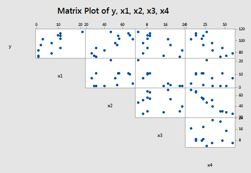
you can get a hunch of which predictors are good candidates for being the first to enter the stepwise model. It looks as if the strongest relationship exists between either \(y\) and \(x_{2} \) or between \(y\) and \(x_{4} \) — and therefore, perhaps either \(x_{2} \) or \(x_{4} \) should enter the stepwise model first. Did you notice what else is going on in this data set though? A strong correlation also exists between the predictors \(x_{2} \) and \(x_{4} \) ! How does this correlation among the predictor variables play out in the stepwise procedure? Let's see what happens when we use the stepwise regression method to find a model that is appropriate for these data.
The procedure
Again, before we learn the finer details, let me again provide a broad overview of the steps involved. First, we start with no predictors in our "stepwise model." Then, at each step along the way we either enter or remove a predictor based on the partial F-tests — that is, the t-tests for the slope parameters — that are obtained. We stop when no more predictors can be justifiably entered or removed from our stepwise model, thereby leading us to a "final model."
Now, let's make this process a bit more concrete. Here goes:
Starting the procedure
The first thing we need to do is set a significance level for deciding when to enter a predictor into the stepwise model. We'll call this the Alpha-to-Enter significance level and will denote it as \(\alpha_{E} \). Of course, we also need to set a significance level for deciding when to remove a predictor from the stepwise model. We'll call this the Alpha-to-Remove significance level and will denote it as \(\alpha_{R} \). That is, first:
- Specify an Alpha-to-Enter significance level. This will typically be greater than the usual 0.05 level so that it is not too difficult to enter predictors into the model. Many software packages — Minitab included — set this significance level by default to \(\alpha_E = 0.15\).
- Specify an Alpha-to-Remove significance level. This will typically be greater than the usual 0.05 level so that it is not too easy to remove predictors from the model. Again, many software packages — Minitab included — set this significance level by default to \(\alpha_{R} = 0.15\).
Step #1:
Once we've specified the starting significance levels, then we:
- Fit each of the one-predictor models — that is, regress \(y\) on \(x_{1} \), regress \(y\) on \(x_{2} \), ..., and regress \(y\) on \(x_{p-1} \).
- Of those predictors whose t-test P-value is less than \(\alpha_E = 0.15\), the first predictor put in the stepwise model is the predictor that has the smallest t-test P-value.
- If no predictor has a t-test P-value less than \(\alpha_E = 0.15\), stop.
Step #2:
Then:
- Suppose \(x_{1} \) had the smallest t-test P-value below \(\alpha_{E} = 0.15\) and therefore was deemed the "best" single predictor arising from the first step.
- Now, fit each of the two-predictor models that include \(x_{1} \) as a predictor — that is, regress \(y\) on \(x_{1} \) and \(x_{2} \) , regress \(y\) on \(x_{1} \) and \(x_{3} \) , ..., and regress \(y\) on \(x_{1} \) and \(x_{p-1} \) .
- Of those predictors whose t-test P-value is less than \(\alpha_E = 0.15\), the second predictor put in the stepwise model is the predictor that has the smallest t-test P-value.
- If no predictor has a t-test P-value less than \(\alpha_E = 0.15\), stop. The model with the one predictor obtained from the first step is your final model.
- But, suppose instead that \(x_{2} \) was deemed the "best" second predictor and it is therefore entered into the stepwise model.
- Now, since \(x_{1} \) was the first predictor in the model, step back and see if entering \(x_{2} \) into the stepwise model somehow affected the significance of the \(x_{1} \) predictor. That is, check the t-test P-value for testing \(\beta_{1}= 0\). If the t-test P-value for \(\beta_{1}= 0\) has become not significant — that is, the P-value is greater than \(\alpha_{R} \) = 0.15 — remove \(x_{1} \) from the stepwise model.
Step #3
Then:
- Suppose both \(x_{1} \) and \(x_{2} \) made it into the two-predictor stepwise model and remained there.
- Now, fit each of the three-predictor models that include \(x_{1} \) and \(x_{2} \) as predictors — that is, regress \(y\) on \(x_{1} \) , \(x_{2} \) , and \(x_{3} \) , regress \(y\) on \(x_{1} \) , \(x_{2} \) , and \(x_{4} \) , ..., and regress \(y\) on \(x_{1} \) , \(x_{2} \) , and \(x_{p-1} \) .
- Of those predictors whose t-test P-value is less than \(\alpha_E = 0.15\), the third predictor put in the stepwise model is the predictor that has the smallest t-test P-value.
- If no predictor has a t-test P-value less than \(\alpha_E = 0.15\), stop. The model containing the two predictors obtained from the second step is your final model.
- But, suppose instead that \(x_{3} \) was deemed the "best" third predictor and it is therefore entered into the stepwise model.
- Now, since \(x_{1} \) and \(x_{2} \) were the first predictors in the model, step back and see if entering \(x_{3} \) into the stepwise model somehow affected the significance of the \(x_{1 } \) and \(x_{2} \) predictors. That is, check the t-test P-values for testing \(\beta_{1} = 0\) and \(\beta_{2} = 0\). If the t-test P-value for either \(\beta_{1} = 0\) or \(\beta_{2} = 0\) has become not significant — that is, the P-value is greater than \(\alpha_{R} = 0.15\) — remove the predictor from the stepwise model.
Stopping the procedure
Continue the steps as described above until adding an additional predictor does not yield a t-test P-value below \(\alpha_E = 0.15\).
Whew! Let's return to our cement data example so we can try out the stepwise procedure as described above.
Back to the example...
To start our stepwise regression procedure, let's set our Alpha-to-Enter significance level at \(\alpha_{E} \) = 0.15, and let's set our Alpha-to-Remove significance level at \(\alpha_{R} = 0.15\). Now, regressing \(y\) on \(x_{1} \) , regressing \(y\) on \(x_{2} \) , regressing \(y\) on \(x_{3} \) , and regressing \(y\) on \(x_{4} \) , we obtain:
Predictor | Coef | SE Coef | T | P |
|---|---|---|---|---|
Constant | 81.479 | 4.927 | 16.54 | 0.000 |
x1 | 1.8687 | 0.5264 | 3.55 | 0.005 |
Predictor | Coef | SE Coef | T | P |
|---|---|---|---|---|
Constant | 57.424 | 8.491 | 6.76 | 0.000 |
x2 | 0.7891 | 0.1684 | 4.69 | 0.001 |
Predictor | Coef | SE Coef | T | P |
|---|---|---|---|---|
Constant | 110.203 | 7.948 | 13.87 | 0.000 |
x3 | -1.2558 | 0.5984 | -2.10 | 0.060 |
Predictor | Coef | SE Coef | T | P |
|---|---|---|---|---|
Constant | 117.568 | 5.262 | 22.34 | 0.000 |
x4 | -0.7382 | 0.1546 | -4.77 | 0.001 |
Each of the predictors is a candidate to be entered into the stepwise model because each t-test P-value is less than \(\alpha_E = 0.15\). The predictors \(x_{2} \) and \(x_{4} \) tie for having the smallest t-test P-value — it is 0.001 in each case. But note the tie is an artifact of Minitab rounding to three decimal places. The t-statistic for \(x_{4} \) is larger in absolute value than the t-statistic for \(x_{2} \) — 4.77 versus 4.69 — and therefore the P-value for \(x_{4} \) must be smaller. As a result of the first step, we enter \(x_{4} \) into our stepwise model.
Now, following step #2, we fit each of the two-predictor models that include \(x_{4} \) as a predictor — that is, we regress \(y\) on \(x_{4} \) and \(x_{1} \), regress \(y\) on \(x_{4} \) and \(x_{2} \), and regress \(y\) on \(x_{4} \) and \(x_{3} \), obtaining:
Predictor | Coef | SE Coef | T | P |
|---|---|---|---|---|
Constant | 103.097 | 2.124 | 48.54 | 0.000 |
x4 | -0.61395 | 0.04864 | -12.62 | 0.000 |
x1 | 1.4400 | 0.1384 | 10.40 | 0.000 |
Predictor | Coef | SE Coef | T | P |
|---|---|---|---|---|
Constant | 94.16 | 56.63 | 1.66 | 0.127 |
x4 | -0.4569 | 0.6960 | -0.66 | 0.526 |
x2 | 0.3109 | 0.7486 | 0.42 | 0.687 |
Predictor | Coef | SE Coef | T | P |
|---|---|---|---|---|
Constant | 131.282 | 3.275 | 40.09 | 0.000 |
x4 | -0.72460 | 0.07233 | -10.02 | 0.000 |
x3 | -1.1999 | 0.1890 | -6.35 | 0.000 |
The predictor \(x_{2} \) is not eligible for entry into the stepwise model because its t-test P-value (0.687) is greater than \(\alpha_E = 0.15\). The predictors \(x_{1} \) and \(x_{3} \) are candidates because each t-test P-value is less than \(\alpha_{E} \) = 0.15. The predictors \(x_{1} \) and \(x_{3} \) tie for having the smallest t-test P-value — it is < 0.001 in each case. But, again the tie is an artifact of Minitab rounding to three decimal places. The t-statistic for \(x_{1} \) is larger in absolute value than the t-statistic for \(x_{3} \) — 10.40 versus 6.3 5— and therefore the P-value for \(x_{1} \) must be smaller. As a result of the second step, we enter \(x_{1} \) into our stepwise model.
Now, since \(x_{4} \) was the first predictor in the model, we must step back and see if entering \(x_{1} \) into the stepwise model affected the significance of the \(x_{4} \) predictor. It did not — the t-test P-value for testing \(\beta_{1} = 0\) is less than 0.001, and thus smaller than \(\alpha_{R} \) = 0.15. Therefore, we proceed to the third step with both \(x_{1} \) and \(x_{4} \) as predictors in our stepwise model.
Now, following step #3, we fit each of the three-predictor models that include x1 and \(x_{4} \) as predictors — that is, we regress \(y\) on \(x_{4} \), \(x_{1} \), and \(x_{2} \); and we regress \(y\) on \(x_{4} \), \(x_{1} \), and \(x_{3} \), obtaining:
Predictor | Coef | SE Coef | T | P |
|---|---|---|---|---|
Constant | 71.65 | 14.14 | 5.07 | 0.001 |
x4 | -0.2365 | 0.1733 | -1.37 | 0.205 |
x1 | 1.4519 | 0.1170 | 12.41 | 0.000 |
x2 | 0.4161 | 0.1856 | 2.24 | 0.052 |
Predictor | Coef | SE Coef | T | P |
|---|---|---|---|---|
Constant | 111.684 | 4.562 | 24.48 | 0.000 |
x4 | -0.64280 | 0.04454 | -14.43 | 0.000 |
x1 | 1.0519 | 0.2237 | 4.70 | 0.001 |
x3 | -0.4100 | 0.1992 | -2.06 | 0.070 |
Both of the remaining predictors — \(x_{2} \) and \(x_{3} \) — are candidates to be entered into the stepwise model because each t-test P-value is less than \(\alpha_E = 0.15\). The predictor \(x_{2} \) has the smallest t-test P-value (0.052). Therefore, as a result of the third step, we enter \(x_{2} \) into our stepwise model.
Now, since \(x_{1} \) and \(x_{4} \) were the first predictors in the model, we must step back and see if entering \(x_{2} \) into the stepwise model affected the significance of the \(x_{1} \) and \(x_{4} \) predictors. Indeed, it did — the t-test P-value for testing \(\beta_{4} \) = 0 is 0.205, which is greater than \(α_{R} = 0.15\). Therefore, we remove the predictor \(x_{4} \) from the stepwise model, leaving us with the predictors \(x_{1} \) and \(x_{2} \) in our stepwise model:
Predictor | Coef | SE Coef | T | P |
|---|---|---|---|---|
Constant | 52.577 | 2.286 | 23.00 | 0.000 |
x1 | 1.4683 | 0.1213 | 12.10 | 0.000 |
x2 | 0.66225 | 0.04585 | 14.44 | 0.000 |
Now, we proceed to fit each of the three-predictor models that include \(x_{1} \) and \(x_{2} \) as predictors — that is, we regress \(y\) on \(x_{1} \), \(x_{2} \), and \(x_{3} \); and we regress \(y\) on \(x_{1} \), \(x_{2} \), and \(x_{4} \), obtaining:
Predictor | Coef | SE Coef | T | P |
|---|---|---|---|---|
Constant | 71.65 | 14.14 | 5.07 | 0.001 |
x1 | 1.4519 | 0.1170 | 12.41 | 0.000 |
x2 | 0.4161 | 0.1856 | 2.24 | 0.052 |
x4 | -0.2365 | 0.1733 | -1.37 | 0.205 |
Predictor | Coef | SE Coef | T | P |
|---|---|---|---|---|
Constant | 48.194 | 3.913 | 12.32 | 0.000 |
x1 | 1.6959 | 0.2046 | 8.29 | 0.000 |
x2 | 0.65691 | 0.04423 | 14.85 | 0.000 |
x3 | 0.2500 | 0.1847 | 1.35 | 0.209 |
Neither of the remaining predictors — \(x_{3} \) and \(x_{4} \) — are eligible for entry into our stepwise model, because each t-test P-value — 0.209 and 0.205, respectively — is greater than \(\alpha_{E} \) = 0.15. That is, we stop our stepwise regression procedure. Our final regression model, based on the stepwise procedure contains only the predictors \(x_1 \text{ and } x_2 \colon \)
Predictor | Coef | SE Coef | T | P |
|---|---|---|---|---|
Constant | 52.577 | 2.286 | 23.00 | 0.000 |
x1 | 1.4683 | 0.1213 | 12.10 | 0.000 |
x2 | 0.66225 | 0.04585 | 14.44 | 0.000 |
Whew! That took a lot of work! The good news is that most statistical software — including Minitab — provides a stepwise regression procedure that does all of the dirty work for us. For example in Minitab, select Stat > Regression > Regression > Fit Regression Model, click the Stepwise button in the resulting Regression Dialog, select Stepwise for Method, and select Include details for each step under Display the table of model selection details. Here's what the Minitab stepwise regression output looks like for our cement data example:
Stepwise Selection of Terms
Candidate terms: x1, x2, x3, x4
Terms | -----Step 1----- | -----Step 2----- | -----Step 3----- | -----Step 4----- | ||||
|---|---|---|---|---|---|---|---|---|
Coef | P | Coef | P | Coef | P | Coef | P | |
Constant | 117.57 | 103.10 | 71.6 | 52.58 | ||||
x4 | -0.738 | 0.001 | -0.6140 | 0.000 | -0.237 | 0.205 | ||
x1 | 1.440 | 0.000 | 1.452 | 0.000 | 1.468 | 0.000 | ||
x2 | 0.416 | 0.052 | 0.6623 | 0.000 | ||||
S | 8.96390 | 2.73427 | 2.30874 | 2.40634 | ||||
R-sq | 67.45% | 97.25% | 98.23% | 97.44% | ||||
R-sq(adj) | 64.50% | 96.70% | 97.64% | 97.44% | ||||
R-sq(pred) | 56.03% | 95.54% | 96.86% | 96.54% | ||||
Mallows' Cp | 138.73 | 5.50 | 3.02 | 2.68 | ||||
\(\alpha\) to enter =0.15, \(\alpha\) to remove 0.15
Minitab tells us that :
- a stepwise regression procedure was conducted on the response \(y\) and four predictors \(x_{1} \) , \(x_{2} \) , \(x_{3} \) , and \(x_{4} \)
- the Alpha-to-Enter significance level was set at \(\alpha_E = 0.15\) and the Alpha-to-Remove significance level was set at \(\alpha_{R} = 0.15\)
The remaining portion of the output contains the results of the various steps of Minitab's stepwise regression procedure. One thing to keep in mind is that Minitab numbers the steps a little differently than described above. Minitab considers a step any addition or removal of a predictor from the stepwise model, whereas our steps — step #3, for example — consider the addition of one predictor and the removal of another as one step.
The results of each of Minitab's steps are reported in a column labeled by the step number. It took Minitab 4 steps before the procedure was stopped. Here's what the output tells us:
- Just as our work above showed, as a result of Minitab's first step, the predictor \(x_{4} \) is entered into the stepwise model. Minitab tells us that the estimated intercept ("Constant") \(b_{0} \) = 117.57 and the estimated slope \(b_{4} = -0.738\). The P-value for testing \(\beta_{4} \) = 0 is 0.001. The estimate S, which equals the square root of MSE, is 8.96. The \(R^{2} \text{-value}\) is 67.45% and the adjusted \(R^{2} \text{-value}\) is 64.50%. Mallows' Cp-statistic, which we learn about in the next section, is 138.73. The output also includes a predicted \(R^{2} \text{-value}\), which we'll come back to in Section 10.5.
- As a result of Minitab's second step, the predictor \(x_{1} \) is entered into the stepwise model already containing the predictor \(x_{4} \). Minitab tells us that the estimated intercept \(b_{0} = 103.10\), the estimated slope \(b_{4} = -0.614\), and the estimated slope \(b_{1} = 1.44\). The P-value for testing \(\beta_{4} = 0\) is < 0.001. The P-value for testing \(\beta_{1} = 0\) is < 0.001. The estimate S is 2.73. The \(R^{2} \text{-value}\) is 97.25% and the adjusted \(R^{2} \text{-value}\) is 96.70%. Mallows' Cp-statistic is 5.5.
- As a result of Minitab's third step, the predictor \(x_{2} \) is entered into the stepwise model already containing the predictors \(x_{1} \) and \(x_{4} \). Minitab tells us that the estimated intercept \(b_{0} = 71.6\), the estimated slope \(b_{4} \) = -0.237, the estimated slope \(b_{1} = 1.452\), and the estimated slope \(b_{2} = 0.416\). The P-value for testing \(\beta_{4} = 0\) is 0.205. The P-value for testing \(\beta_{1} = 0\) is < 0.001. The P-value for testing \(\beta_{2} = 0\) is 0.052. The estimate S is 2.31. The \(R^{2} \text{-value}\) is 98.23% and the adjusted \(R^{2} \text{-value}\) is 97.64%. Mallows' Cp-statistic is 3.02.
- As a result of Minitab's fourth and final step, the predictor \(x_{4} \) is removed from the stepwise model containing the predictors \(x_{1} \), \(x_{2} \), and \(x_{4} \), leaving us with the final model containing only the predictors \(x_{1} \) and \(x_{2} \). Minitab tells us that the estimated intercept \(b_{0} = 52.58\), the estimated slope \(b_{1} = 1.468\), and the estimated slope \(b_{2} = 0.6623\). The P-value for testing \(\beta_{1} = 0\) is < 0.001. The P-value for testing \(\beta_{2} \) = 0 is < 0.001. The estimate S is 2.41. The \(R^{2} \text{-value}\) is 97.87% and the adjusted \(R^{2} \text{-value}\) is 97.44%. Mallows' Cp-statistic is 2.68.
Does the stepwise regression procedure lead us to the "best" model? No, not at all! Nothing occurs in the stepwise regression procedure to guarantee that we have found the optimal model. Case in point! Suppose we defined the best model to be the model with the largest adjusted \(R^{2} \text{-value}\). Then, here, we would prefer the model containing the three predictors \(x_{1} \), \(x_{2} \), and \(x_{4} \), because its adjusted \(R^{2} \text{-value}\) is 97.64%, which is higher than the adjusted \(R^{2} \text{-value}\) of 97.44% for the final stepwise model containing just the two predictors \(x_{1} \) and \(x_{2} \).
Again, nothing occurs in the stepwise regression procedure to guarantee that we have found the optimal model. This, and other cautions of the stepwise regression procedure, are delineated in the next section.
Cautions!
Here are some things to keep in mind concerning the stepwise regression procedure:
- The final model is not guaranteed to be optimal in any specified sense.
- The procedure yields a single final model, although there are often several equally good models.
- Stepwise regression does not take into account a researcher's knowledge about the predictors. It may be necessary to force the procedure to include important predictors.
- One should not over-interpret the order in which predictors are entered into the model.
- One should not jump to the conclusion that all the important predictor variables for predicting \(y\) have been identified, or that all the unimportant predictor variables have been eliminated. It is, of course, possible that we may have committed a Type I or Type II error along the way.
- Many t-tests for testing \(\beta_{k} = 0\) are conducted in a stepwise regression procedure. The probability is therefore high that we included some unimportant predictors or excluded some important predictors.
It's for all of these reasons that one should be careful not to overuse or overstate the results of any stepwise regression procedure.
Example 10-2: Blood Pressure
Some researchers observed the following data (Blood pressure dataset) on 20 individuals with high blood pressure:
- blood pressure (\(y = BP \), in mm Hg)
- age (\(x_{1} = \text{Age} \), in years)
- weight (\(x_{2} = \text{Weight} \), in kg)
- body surface area (\(x_{3} = \text{BSA} \), in sq m)
- duration of hypertension ( \(x_{4} = \text{Dur} \), in years)
- basal pulse (\(x_{5} = \text{Pulse} \), in beats per minute)
- stress index (\(x_{6} = \text{Stress} \) )
The researchers were interested in determining if a relationship exists between blood pressure and age, weight, body surface area, duration, pulse rate, and/or stress level.
The matrix plot of BP, Age, Weight, and BSA looks like this:
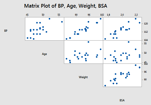
and the matrix plot of BP, Dur, Pulse, and Stress looks like this:

Using Minitab to perform the stepwise regression procedure, we obtain:
Stepwise Selection of Terms
Candidate terms: Age, Weight, BSA, Pulse, Stress
Terms | -----Step 1----- | -----Step 2----- | -----Step 3----- | |||
|---|---|---|---|---|---|---|
Coef | P | Coef | P | Coef | P | |
Constant | 2.21 | -16.58 | -13.67 | |||
Weight | 1.2009 | 0.000 | 1.0330 | 0.000 | 0.9058 | 0.000 |
Age | 0.7083 | 0.000 | 0.7016 | 0.008 | ||
BSA | 4.63 | 0.008 | ||||
S | 1.74050 | 0.532692 | 0.437046 | |||
R-sq | 90.26% | 99.14% | 99.45% | |||
R-sq(adj) | 89.72% | 99.04% | 99.35% | |||
R-sq(pred) | 88.53% | 98.89% | 99.22% | |||
Mallows' Cp | 312.81 | 15.09 | 6.43 | |||
\(\alpha\) to enter =0.15, \(\alpha\) to remove 0.15
When \( \alpha_{E} = \alpha_{R} = 0.15\), the final stepwise regression model contains the predictors of Weight, Age, and BSA.
The following video will walk through this example in Minitab.
Try it!
Stepwise regression
Brain size and body size. Imagine that you do not have automated stepwise regression software at your disposal, and conduct the stepwise regression procedure on the IQ size data set. Setting Alpha-to-Remove and Alpha-to-Enter at 0.15, verify the final model obtained above by Minitab.
That is:
- First, fit each of the three possible simple linear regression models. That is, regress PIQ on Brain, regress PIQ on Height, and regress PIQ on Weight. (See Minitab Help: Performing a basic regression analysis). The first predictor that should be entered into the stepwise model is the predictor with the smallest P-value (or equivalently the largest t-statistic in absolute value) for testing \(\beta_{k} = 0\), providing the P-value is smaller than 0.15. What is the first predictor that should be entered into the stepwise model?
a. Fit individual models.
PIQ vs Brain, PIQ vs Height, and PIG vs Weight.
b. Include the predictor with the smallest p-value < \(\alpha_E = 0.15\) and largest |T| value.
Include Brain as the first predictor since its p-value = 0.019 is the smallest.
Term
Coef
SE Coef
T-Value
P-Value
Constant
4.7
43.7
0.11
0.916
Brain
1.177
0.481
2.45
0.019
Term
Coef
SE Coef
T-Value
P-Value
Constant
147.4
64.3
2.29
0.028
Height
-0.527
0.939
-0.56
0.578
Term
Coef
SE Coef
T-Value
P-Value
Constant
111.0
24.5
4.53
0.000
Weight
0.002
0.160
0.02
0.988
- Now, fit each of the possible two-predictor multiple linear regression models which include the first predictor identified above and each of the remaining two predictors. (See Minitab Help: Performing a basic regression analysis). Which predictor should be entered into the model next?
a. Fit two predictor models by adding each remaining predictor one at a time.
Fit PIQ vs Brain, Height, and PIQ vs Brain, Weight.
b. Add to the model the 2nd predictor with smallest p-value < \(\alpha_E = 0.15\) and largest |T| value.
Add Height since its p-value = 0.009 is the smallest.
c. Omit any previously added predictors if their p-value exceeded \(\alpha_R = 0.15\)
The previously added predictor Brain is retained since its p-value is still below \(\alpha_R\).
FINAL RESULT of step 2: The model includes the two predictors Brain and Height.
Term
Coef
SE Coef
T-Value
P-Value
Constant
111.3
55.9
1.99
0.054
Brain
2.061
0.547
3.77
0.001
Height
-2.730
0.993
-2.75
0.009
Term
Coef
SE Coef
T-Value
P-Value
Constant
4.8
43.0
0.11
0.913
Brain
1.592
0.551
2.89
0.007
Weight
-0.250
0.170
-1.47
0.151
Term
Coef
SE Coef
T-Value
P-Value
Constant
111.0
24.5
4.53
0.000
Weight
0.002
0.160
0.02
0.988
- Continue the stepwise regression procedure until you can not justify entering or removing any more predictors. What is the final model identified by your stepwise regression procedure?
Fit three predictor models by adding each remaining predictor one at a time.
Run PIQ vs Brain, Height, Weight - weight is the only 3rd predictor.
Add to the model the 3rd predictor with the smallest p-value < \( \alpha_E\) and largest |T| value.
Do not add weight since its p-value \(p = 0.998 > \alpha_E = 0.15\)
Term
Coef
SE Coef
T-Value
P-Value
Constant
111.4
63.0
1.77
0.086
Brain
2.060
0.563
3.66
0.001
Height
-2.73
1.23
-2.22
0.033
Weight
0.001
0.197
0.00
0.998
Omit any previously added predictors if their p-value exceeded \(\alpha_R\).
The previously added predictors Brain and Height are retained since their p-values are both still below \(\alpha_R\).
Term
Coef
SE Coef
T-Value
P-Value
Constant
111.3
55.9
1.99
0.054
Brain
2.061
0.547
3.77
0.001
Height
-2.730
0.993
-2.75
0.009
The final model contains the two predictors, Brain and Height.
10.3 - Best Subsets Regression, Adjusted R-Sq, Mallows Cp
10.3 - Best Subsets Regression, Adjusted R-Sq, Mallows CpIn this section, we learn about the best subsets regression procedure (also known as the all possible subsets regression procedure). While we will soon learn the finer details, the general idea behind best subsets regression is that we select the subset of predictors that do the best at meeting some well-defined objective criterion, such as having the largest \(R^{2} \text{-value}\) or the smallest MSE.
Again, our hope is that we end up with a reasonable and useful regression model. There is one sure way of ending up with a model that is certain to be underspecified — and that's if the set of candidate predictor variables doesn't include all of the variables that actually predict the response. Therefore, just as is the case for the stepwise regression procedure, a fundamental rule of the best subsets regression procedure is that the list of candidate predictor variables must include all of the variables that actually predict the response. Otherwise, we are sure to end up with a regression model that is underspecified and therefore misleading.
The procedure
A regression analysis utilizing the best subsets regression procedure involves the following steps:
Step #1
First, identify all of the possible regression models derived from all of the possible combinations of the candidate predictors. Unfortunately, this can be a huge number of possible models.
For the sake of example, suppose we have three (3) candidate predictors — \(x_{1}\), \(x_{2}\), and \(x_{3}\)— for our final regression model. Then, there are eight (8) possible regression models we can consider:
- the one (1) model with no predictors
- the three (3) models with only one predictor each — the model with \(x_{1}\) alone; the model with \(x_{2}\) alone; and the model with \(x_{3}\) alone
- the three (3) models with two predictors each — the model with \(x_{1}\) and \(x_{2}\); the model with \(x_{1}\) and \(x_{3}\); and the model with \(x_{2}\) and \(x_{3}\)
- and the one (1) model with all three predictors — that is, the model with \(x_{1}\), \(x_{2}\) and \(x_{3}\)
That's 1 + 3 + 3 + 1 = 8 possible models to consider. It can be shown that when there are four candidate predictors — \(x_{1}\), \(x_{2}\), \(x_{3}\) and \(x_{4}\) — there are 16 possible regression models to consider. In general, if there are p-1 possible candidate predictors, then there are \(2^{p-1}\) possible regression models containing the predictors. For example, 10 predictors yield \(2^{10} = 1024\) possible regression models.
That's a heck of a lot of models to consider! The good news is that statistical software, such as Minitab, does all of the dirty work for us.
Step #2
From the possible models identified in the first step, determine the one-predictor models that do the "best" at meeting some well-defined criteria, the two-predictor models that do the "best," the three-predictor models that do the "best," and so on. For example, suppose we have three candidate predictors — \(x_{1}\), \(x_{2}\), and \(x_{3}\) — for our final regression model. Of the three possible models with one predictor, identify the one or two that do "best." Of the three possible two-predictor models, identify the one or two that do "best." By doing this, it cuts down considerably the number of possible regression models to consider!
But, have you noticed that we have not yet even defined what we mean by "best"? What do you think "best" means? Of course, you'll probably define it differently than me or than your neighbor. Therein lies the rub — we might not be able to agree on what's best! In thinking about what "best" means, you might have thought of any of the following:
- the model with the largest \(R^{2}\)
- the model with the largest adjusted \(R^{2}\)
- the model with the smallest MSE (or S = square root of MSE)
There are other criteria you probably didn't think of, but we could consider, too, for example, Mallows' \(C_{p}\)-statistic, the PRESS statistic, and Predicted \(R^{2}\) (which is calculated from the PRESS statistic). We'll learn about Mallows' \(C_{p}\)-statistic in this section and about the PRESS statistic and Predicted \(R^{2}\) in Section 10.5.
To make matters even worse — the different criteria quantify different aspects of the regression model, and therefore often yield different choices for the best set of predictors. That's okay — as long as we don't misuse best subsets regression by claiming that it yields the best model. Rather, we should use best subsets regression as a screening tool — that is, as a way to reduce a large number of possible regression models to just a handful of models that we can evaluate further before arriving at one final model.
Step #3
Further, evaluate and refine the handful of models identified in the last step. This might entail performing residual analyses, transforming the predictors and/or responses, adding interaction terms, and so on. Do this until you are satisfied that you have found a model that meets the model conditions, does a good job of summarizing the trend in the data, and most importantly allows you to answer your research question.
Example 10-3: Cement Data
For the remainder of this section, we discuss how the criteria identified above can help us reduce a large number of possible regression models to just a handful of models suitable for further evaluation.
For the sake of an example, we will use the cement data to illustrate the use of the criteria. Therefore, let's quickly review — the researchers measured and recorded the following data (Cement data) on 13 batches of cement:
- Response y: heat evolved in calories during the hardening of cement on a per-gram basis
- Predictor \(x_{1}\): % of tricalcium aluminate
- Predictor \(x_{2}\): % of tricalcium silicate
- Predictor \(x_{3}\): % of tetra calcium alumino ferrite
- Predictor \(x_{4}\): % of dicalcium silicate
And, the matrix plot of the data looks like this:
The \(R^{2} \text{-values}\)
As you may recall, the \(R^{2} \text{-value}\), which is defined as:
\(R^2=\dfrac{SSR}{SSTO}=1-\dfrac{SSE}{SSTO}\)
can only increase as more variables are added. Therefore, it makes no sense to define the "best" model as the model with the largest \(R^{2} \text{-value}\). After all, if we did, the model with the largest number of predictors would always win.
All is not lost, however. We can instead use the \(R^{2} \text{-values}\) to find the point where adding more predictors is not worthwhile, because it yields a very small increase in the \(R^{2}\)-value. In other words, we look at the size of the increase in \(R^{2}\), not just its magnitude alone. Because this is such a "wishy-washy" criterion, it is used most often in combination with the other criteria.
Let's see how this criterion works in the cement data example. In doing so, you get your first glimpse of Minitab's best subsets regression output. For Minitab, select Stat > Regression > Regression > Best Subsets to do a best subsets regression.
Best Subsets Regressions: y versus x1, x2, x3, x4
Response is y
Vars | R-Sq | R-Sq | R-Sq | Mallows | S | x | x | x | x |
|---|---|---|---|---|---|---|---|---|---|
1 | 2 | 3 | 4 | ||||||
1 | 67.5 | 64.5 | 56.0 | 138.7 | 8.9639 | X | |||
1 | 66.6 | 63.6 | 55.7 | 142.5 | 9.0771 | X | |||
2 | 97.9 | 97.4 | 96.5 | 2.7 | 2.4063 | X | X | ||
2 | 97.2 | 96.7 | 95.5 | 5.5 | 2.7343 | X | X | ||
3 | 98.2 | 97.6 | 96.9 | 3.0 | 2.3087 | X | X | X | |
3 | 98.2 | 97.6 | 96.7 | 3.0 | 2.3232 | X | X | X | |
4 | 98.2 | 97.4 | 95.9 | 5.0 | 2.4460 | X | X | X | X |
Each row in the table represents information about one of the possible regression models. The first column — labeled Vars — tells us how many predictors are in the model. The last four columns — labeled downward x1, x2, x3, and x4 — tell us which predictors are in the model. If an "X" is present in the column, then that predictor is in the model. Otherwise, it is not. For example, the first row in the table contains information about the model in which \(x_{4}\) is the only predictor, whereas the fourth row contains information about the model in which \(x_{1}\) and \(x_{4}\) are the two predictors in the model. The other five columns — labeled R-sq, R-sq(adj), R-sq(pred), Cp, and S — pertain to the criteria that we use in deciding which models are "best."
As you can see, by default Minitab reports only the two best models for each number of predictors based on the size of the \(R^{2} \text{-value}\) that is, Minitab reports the two one-predictor models with the largest \(R^{2} \text{-values}\), followed by the two two-predictor models with the largest \(R^{2} \text{-values}\), and so on.
So, using the \(R^{2} \text{-value}\) criterion, which model (or models) should we consider for further evaluation? Hmmm — going from the "best" one-predictor model to the "best" two-predictor model, the \(R^{2} \text{-value}\) jumps from 67.5 to 97.9. That is a jump worth making! That is, with such a substantial increase in the \(R^{2} \text{-value}\), one could probably not justify — with a straight face at least — using the one-predictor model over the two-predictor model. Now, should we instead consider the "best" three-predictor model? Probably not! The increase in the \(R^{2} \text{-value}\) is very small — from 97.9 to 98.2 — and therefore, we probably can't justify using the larger three-predictor model over the simpler, smaller two-predictor model. Get it? Based on the \(R^{2} \text{-value}\) criterion, the "best" model is the model with the two predictors \(x_{1}\) and \(x_{2}\).
The adjusted \(R^{2} \text{-value}\) and MSE
The adjusted \(R^{2} \text{-value}\), which is defined as:
\begin{align} R_{a}^{2}&=1-\left(\dfrac{n-1}{n-p}\right)\left(\dfrac{SSE}{SSTO}\right)\\&=1-\left(\dfrac{n-1}{SSTO}\right)MSE\\&=\dfrac{\dfrac{SSTO}{n-1}-\frac{SSE}{n-p}}{\dfrac{SSTO}{n-1}}\end{align}
makes us pay a penalty for adding more predictors to the model. Therefore, we can just use the adjusted \(R^{2} \text{-value}\) outright. That is, according to the adjusted \(R^{2} \text{-value}\) criterion, the best regression model is the one with the largest adjusted \(R^{2}\)-value.
Now, you might have noticed that the adjusted \(R^{2} \text{-value}\) is a function of the mean square error (MSE). And, you may — or may not — recall that MSE is defined as:
\(MSE=\dfrac{SSE}{n-p}=\dfrac{\sum(y_i-\hat{y}_i)^2}{n-p}\)
That is, MSE quantifies how far away our predicted responses are from our observed responses. Naturally, we want this distance to be small. Therefore, according to the MSE criterion, the best regression model is the one with the smallest MSE.
But, aha — the two criteria are equivalent! If you look at the formula again for the adjusted \(R^{2} \text{-value}\):
\(R_{a}^{2}=1-\left(\dfrac{n-1}{SSTO}\right)MSE\)
you can see that the adjusted \(R^{2} \text{-value}\) increases only if MSE decreases. That is, the adjusted \(R^{2} \text{-value}\) and MSE criteria always yield the same "best" models.
Back to the cement data example! One thing to note is that S is the square root of MSE. Therefore, finding the model with the smallest MSE is equivalent to finding the model with the smallest S:
Best Subsets Regressions: y versus x1 ,x2, x3, x4
Response is y
Vars | R-Sq | R-Sq | R-Sq | Mallows | S | x | x | x | x |
|---|---|---|---|---|---|---|---|---|---|
1 | 2 | 3 | 4 | ||||||
1 | 67.5 | 64.5 | 56.0 | 138.7 | 8.9639 | X | |||
1 | 66.6 | 63.6 | 55.7 | 142.5 | 9.0771 | X | |||
2 | 97.9 | 97.4 | 96.5 | 2.7 | 2.4063 | X | X | ||
2 | 97.2 | 96.7 | 95.5 | 5.5 | 2.7343 | X | X | ||
3 | 98.2 | 97.6 | 96.9 | 3.0 | 2.3087 | X | X | X | |
3 | 98.2 | 97.6 | 96.7 | 3.0 | 2.3232 | X | X | X | |
4 | 98.2 | 97.4 | 95.9 | 5.0 | 2.4460 | X | X | X | X |
The model with the largest adjusted \(R^{2} \text{-value}\) (97.6) and the smallest S (2.3087) is the model with the three predictors \(x_{1}\), \(x_{2}\), and \(x_{4}\).
See?! Different criteria can indeed lead us to different "best" models. Based on the \(R^{2} \text{-value}\) criterion, the "best" model is the model with the two predictors \(x_{1}\) and \(x_{2}\). But, based on the adjusted \(R^{2} \text{-value}\) and the smallest MSE criteria, the "best" model is the model with the three predictors \(x_{1}\), \(x_{2}\), and \(x_{4}\).
Mallows' \(C_{p}\)-statistic
Recall that an underspecified model is a model in which important predictors are missing. And, an underspecified model yields biased regression coefficients and biased predictions of the response. Well, in short, Mallows' \(C_{p}\)-statistic estimates the size of the bias that is introduced into the predicted responses by having an underspecified model.
Now, we could just jump right in and be told how to use Mallows' \(C_{p}\)-statistic as a way of choosing a "best" model. But, then it wouldn't make any sense to you — and therefore it wouldn't stick to your craw. So, we'll start by justifying the use of the Mallows' \(C_{p}\)-statistic. The problem is it's kind of complicated. So, be patient, don't be frightened by the scary-looking formulas, and before you know it, we'll get to the moral of the story. Oh, and by the way, in case you're wondering — it's called Mallows' \(C_{p}\)-statistic, because a guy named Mallows thought of it!
Here goes! At issue in any regression model are two things, namely:
- The bias in the predicted responses.
- The variation in the predicted responses.
Bias in predicted responses
Recall that, in fitting a regression model to data, we attempt to estimate the average — or expected value — of the observed responses \(E \left( y_i \right) \) at any given predictor value x. That is, \(E \left( y_i \right) \) is the population regression function. Because the average of the observed responses depends on the value of x, we might also denote this population average or population regression function as \(\mu_{Y|x}\).
Now, if there is no bias in the predicted responses, then the average of the observed responses \(E \left( y_i \right) \) and the average of the predicted responses E(\(\hat{y}_i\)) both equal the thing we are trying to estimate, namely the average of the responses in the population \(\mu_{Y|x}\). On the other hand, if there is bias in the predicted responses, then \(E \left( y_i \right) \) = \(\mu_{Y|x}\) and E(\(\hat{y}_i\)) do not equal each other. The difference between \(E \left( y_i \right) \) and E(\(\hat{y}_i\)) is the bias \(B_i\) in the predicted response. That is, the bias:
\(B_i=E(\hat{y}_i) - E(y_i)\)
We can picture this bias as follows:
The quantity \(E \left( y_i \right) \) is the value of the population regression line at a given x. Recall that we assume that the error terms \(\epsilon_i\) are normally distributed. That's why there is a normal curve — in red — drawn around the population regression line \(E \left( y_i \right) \). You can think of the quantity E(\(\hat{y}_i\)) as being the predicted regression line — well, technically, it's the average of all of the predicted regression lines you could obtain based on your formulated regression model. Again, since we always assume the error terms \(\epsilon_i\) are normally distributed, we've drawn a normal curve — in blue— around the average predicted regression line E(\(\hat{y}_i\)). The difference between the population regression line \(E \left( y_i \right) \) and the average predicted regression line E(\(\hat{y}_i\)) is the bias \(B_i=E(\hat{y}_i)-E(y_i)\) .
Earlier in this lesson, we saw an example in which bias was likely introduced into the predicted responses because of an underspecified model. The data concerned the heights and weights of Martians. The Martian data set — don't laugh — contains the weights (in g), heights (in cm), and amount of daily water consumption (0, 10, or 20 cups per day) of 12 Martians.
If we regress y = weight on the predictors \(x_{1}\) = height and \(x_{2}\) = water, we obtain the following estimated regression equation:
Regression Equation
\(\widehat{weight} = -1.220 + -.28344 height + 0.11121 water\)
But, if we regress y = weight on only the one predictor \(x_{1}\) = height, we obtain the following estimated regression equation:
Regression Equation
\(\widehat{weight} = -4.14 + 0.2889 height\)
A plot of the data containing the two estimated regression equations looks like this:
The three black lines represent the estimated regression equation when the amount of water consumption is taken into account — the first line for 0 cups per day, the second line for 10 cups per day, and the third line for 20 cups per day. The dashed blue line represents the estimated regression equation when we leave the amount of water consumed out of the regression model.
As you can see, if we use the blue line to predict the weight of a randomly selected martian, we would consistently overestimate the weight of Martians who drink 0 cups of water a day, and we would consistently underestimate the weight of Martians who drink 20 cups of water a day. That is, our predicted responses would be biased.
Variation in predicted responses
When a bias exists in the predicted responses, the variance in the predicted responses for a data point i is due to two things:
- the ever-present random sampling variation, that is \((\sigma_{\hat{y}_i}^{2})\)
- the variance associated with the bias, that is \((B_{i}^{2})\)
Now, if our regression model is biased, it doesn't make sense to consider the bias at just one data point i. We need to consider the bias that exists for all n data points. Looking at the plot of the two estimated regression equations for the martian data, we see that the predictions for the underspecified model are more biased for certain data points than for others. And, we can't just consider the variation in the predicted responses at one data point i. We need to consider the total variation in the predicted responses.
To quantify the total variation in the predicted responses, we just sum the two variance components — \((\sigma_{\hat{y}_i}^{2})\) and \((B_{i}^{2})\) — over all n data points to obtain a (standardized) measure of the total variation in the predicted responses \(\Gamma_p\) (that's the greek letter "gamma"):
\(\Gamma_p=\dfrac{1}{\sigma^2} \left\{ \sum_{i=1}^{n}\sigma_{\hat{y}_i}^{2}+\sum_{i=1}^{n}\left( E(\hat{y}_i)-E(y_i) \right) ^2 \right\}\)
I warned you about not being overwhelmed by scary-looking formulas! The first term in the brackets quantifies the random sampling variation summed over all n data points, while the second term in the brackets quantifies the amount of bias (squared) summed over all n data points. Because the size of the bias depends on the measurement units used, we divide by \(\sigma^{2}\) to get a standardized unitless measure.
Now, we don't have the tools to prove it, but it can be shown that if there is no bias in the predicted responses — that is, if the bias = 0 — then \(\Gamma_p\) achieves its smallest possible value, namely p, the number of parameters:
\(\Gamma_p=\dfrac{1}{\sigma^2} \left\{ \sum_{i=1}^{n}\sigma_{\hat{y}_i}^{2}+0 \right\} =p\)
Now, because it quantifies the amount of bias and variance in the predicted responses, \(\Gamma_p\) seems to be a good measure of an underspecified model:
\(\Gamma_p=\dfrac{1}{\sigma^2} \left\{ \sum_{i=1}^{n}\sigma_{\hat{y}_i}^{2}+\sum_{i=1}^{n} \left( E(\hat{y}_i)-E(y_i) \right) ^2 \right\}\)
The best model is simply the model with the smallest value of \(\Gamma_p\). We even know that the theoretical minimum of \(\Gamma_p\) is the number of parameters p.
Well, it's not quite that simple — we still have a problem. Did you notice all of those greek parameters — \(\sigma^{2}\), \((\sigma_{\hat{y}_i}^{2})\), and \(\gamma_p\)? As you know, greek parameters are generally used to denote unknown population quantities. That is, we don't or can't know the value of \(\Gamma_p\) — we must estimate it. That's where Mallows' \(C_{p}\)-statistic comes into play!
\(C_{p}\) as an estimate of \(\Gamma_p\)
If we know the population variance \(\sigma^{2}\), we can estimate \(\Gamma_{p}\):
\(C_p=p+\dfrac{(MSE_p-\sigma^2)(n-p)}{\sigma^2}\)
where \(MSE_{p}\) is the mean squared error from fitting the model containing the subset of p-1 predictors (which with the intercept contains p parameters).
But we don't know \(\sigma^{2}\). So, we estimate it using \(MSE_{all}\), the mean squared error obtained from fitting the model containing all of the candidate predictors. That is:
\(C_p=p+\dfrac{(MSE_p-MSE_{all})(n-p)}{MSE_{all}}=\dfrac{SSE_p}{MSE_{all}}-(n-2p)\)
A couple of things to note though. Estimating \(\sigma^{2}\) using \(MSE_{all}\):
- assumes that there are no biases in the full model with all of the predictors, an assumption that may or may not be valid, but can't be tested without additional information (at the very least you have to have all of the important predictors involved)
- guarantees that \(C_{p}\) = p for the full model because in that case \(MSE_{p}\) - \(MSE_{all}\) = 0.
Using the \(C_{p}\) criterion to identify "best" models
Finally — we're getting to the moral of the story! Just a few final facts about Mallows' \(C_{p}\)-statistic will get us on our way. Recalling that p denotes the number of parameters in the model:
- Subset models with small \(C_{p}\) values have a small total (standardized) variance of prediction.
- When the \(C_{p}\) value is ...
- ... near p, the bias is small (next to none)
- ... much greater than p, the bias is substantial
- ... below p, it is due to sampling error; interpret as no bias
- For the largest model containing all of the candidate predictors, \(C_{p}\) = p (always). Therefore, you shouldn't use \(C_{p}\) to evaluate the fullest model.
That all said, here's a reasonable strategy for using \(C_{p}\) to identify "best" models:
- Identify subsets of predictors for which the \(C_{p}\) value is near p (if possible).
- The full model always yields \(C_{p}\)= p, so don't select the full model based on \(C_{p}\).
- If all models, except the full model, yield a large \(C_{p}\) not near p, it suggests some important predictor(s) are missing from the analysis. In this case, we are well-advised to identify the predictors that are missing!
- If several models have \(C_{p}\) near p, choose the model with the smallest \(C_{p}\) value, thereby insuring that the combination of the bias and the variance is at a minimum.
- When more than one model has a small value of \(C_{p}\) value near p, in general, choose the simpler model or the model that meets your research needs.
Example 10-3: Cement Data Continued
Ahhh—an example! Let's see what model the \(C_{p}\) criterion leads us to for the cement data:
Best Subsets Regressions: y versus x1, x2, x3, x4
Response is y
Vars | R-Sq | R-Sq | R-Sq | Mallows | S | x | x | x | x |
|---|---|---|---|---|---|---|---|---|---|
1 | 2 | 3 | 4 | ||||||
1 | 67.5 | 64.5 | 56.0 | 138.7 | 8.9639 | X | |||
1 | 66.6 | 63.6 | 55.7 | 142.5 | 9.0771 | X | |||
2 | 97.9 | 97.4 | 96.5 | 2.7 | 2.4063 | X | X | ||
2 | 97.2 | 96.7 | 95.5 | 5.5 | 2.7343 | X | X | ||
3 | 98.2 | 97.6 | 96.9 | 3.0 | 2.3087 | X | X | X | |
3 | 98.2 | 97.6 | 96.7 | 3.0 | 2.3232 | X | X | X | |
4 | 98.2 | 97.4 | 95.9 | 5.0 | 2.4460 | X | X | X | X |
The first thing you might want to do here is "pencil in" a column to the left of the Vars column. Recall that this column tells us the number of predictors (p-1) that are in the model. But, we need to compare \(C_{p}\) to the number of parameters (p). There is always one more parameter—the intercept parameter—than predictors. So, you might want to add—at least mentally—a column containing the number of parameters—here, 2, 2, 3, 3, 4, 4, and 5.
Here, the model in the third row (containing predictors \(x_{1}\) and \(x_{2}\)), the model in the fifth row (containing predictors \(x_{1}\), \(x_{2}\) and \(x_{4}\)), and the model in the sixth row (containing predictors \(x_{1}\), \(x_{2}\) and \(x_{3}\)) are all unbiased models, because their \(C_{p}\) values equal (or are below) the number of parameters p. For example:
- the model containing the predictors \(x_{1}\) and \(x_{2}\) contains 3 parameters and its \(C_{p}\) value is 2.7. When \(C_{p}\) is less than p, it suggests the model is unbiased;
- the model containing the predictors \(x_{1}\), \(x_{2}\) and \(x_{4}\) contains 4 parameters and its \(C_{p}\) value is 3.0. When \(C_{p}\) is less than p, it suggests the model is unbiased;
- the model containing the predictors \(x_{1}\), \(x_{2}\) and \(x_{3}\) contains 4 parameters and its \(C_{p}\) value is 3.0. When \(C_{p}\) is less than p, it suggests the model is unbiased.
So, in this case, based on the \(C_{p}\) criterion, the researcher has three legitimate models from which to choose with respect to bias. Of these three, the model containing the predictors \(x_{1}\) and \(x_{2}\) has the smallest \(C_{p}\) value, but the \(C_{p}\) values for the other two models are similar and so there is little to separate these models based on this criterion.
Incidentally, you might also want to conclude that the last model — the model containing all four predictors — is a legitimate contender because \(C_{p}\) = 5.0 equals p = 5. Don't forget that the model with all of the predictors is assumed to be unbiased. Therefore, you should not use the \(C_{p}\) criterion as a way of evaluating the fullest model with all of the predictors.
Incidentally, how did Minitab determine that the \(C_{p}\) value for the third model is 2.7, while for the fourth model the \(C_{p}\) value is 5.5? We can verify these calculated \(C_{p}\) values!
The following output was obtained by first regressing y on the predictors \(x_{1}\), \(x_{2}\), \(x_{3}\) and \(x_{4}\) and then by regressing y on the predictors \(x_{1}\) and \(x_{2}\):
Regression Equation
\(\widehat{y} = 62.4 + 1.55 x1 + 0.51 x2 + 0.102 x3 - 0.144 x4\)
Source | DF | SS | MS | F | P |
|---|---|---|---|---|---|
Regression | 4 | 2667.90 | 666.97 | 111.48 | 0.000 |
Residual Error | 8 | 47.86 | 5.98 | ||
Total | 12 | 2715.76 |
Regression Equation
\(\widehat{y} = 52.6 + 1.47 x1 + 0.662 x2\)
Source | DF | SS | MS | F | P |
|---|---|---|---|---|---|
Regression | 2 | 2657.9 | 1328.9 | 229.50 | 0.000 |
Residual Error | 10 | 57.9 | 5.8 | ||
Total | 12 | 2715.8 |
tells us that, here, \(MSE_{all}\) = 5.98 and \(MSE_{p}\) = 5.8. Therefore, just as Minitab claims:
\(C_p=p+\dfrac{(MSE_p-MSE_{all})(n-p)}{MSE_{all}}=3+\dfrac{(5.8-5.98)(13-3)}{5.98}=2.7\)
the \(C_{p}\)-statistic equals 2.7 for the model containing the predictors \(x_{1}\) and \(x_{2}\).
And, the following output is obtained by first regressing y on the predictors \(x_{1}\), \(x_{2}\), \(x_{3}\) and \(x_{4}\) and then by regressing y on the predictors \(x_{1}\) and \(x_{4}\):
Regression Equation
\(\widehat{y} = 62.4 + 1.55 x1 + 0.51 x2 + 0.102 x3 - 0.144 x4\)
Source | DF | SS | MS | F | P |
|---|---|---|---|---|---|
Regression | 4 | 2667.90 | 666.97 | 111.48 | 0.000 |
Residual Error | 8 | 47.86 | 5.98 | ||
Total | 12 | 2715.76 |
Regression Equation
\(\widehat{y} = 103 + 1.44 x1 - 0.614 x4\)
Source | DF | SS | MS | F | P |
|---|---|---|---|---|---|
Regression | 2 | 2641.0 | 1320.5 | 176.63 | 0.000 |
Residual Error | 10 | 74.8 | 7.5 | ||
Total | 12 | 2715.8 |
tells us that, here, \(MSE_{all}\) = 5.98 and \(MSE_{p}\) = 7.5. Therefore, just as Minitab claims:
\(C_p=p+\dfrac{(MSE_p-MSE_{all})(n-p)}{MSE_{all}}=3+\dfrac{(7.5-5.98)(13-3)}{5.98}=5.5\)
the \(C_{p}\)-statistic equals 5.5 for the model containing the predictors \(x_{1}\) and \(x_{4}\).
Try it!
Best subsets regression
When there are four candidate predictors — \(x_1\), \(x_2\), \(x_3\) and \(x_4\) — there are 16 possible regression models to consider. Identify the 16 possible models.
The possible predictor sets and the corresponding models are given below:
Predictor Set | model |
|---|---|
None of \(x_1, x_2, x_3, x_4\) | \(E(Y)=\beta_0\) |
\(x_1\) | \(E(Y)=\beta_0+\beta_1 x_1\) |
\(x_2\) | \(E(Y)=\beta_0+\beta_2 x_2\) |
\(x_3\) | \(E(Y)=\beta_0+\beta_3 x_3\) |
\(x_4\) | \(E(Y)=\beta_0+\beta_4 x_4\) |
\(x_1, x_2\) | \(E(Y)=\beta_0+\beta_1 x_1+\beta_2 x_2\) |
\(x_1, x_3\) | \(E(Y)=\beta_0+\beta_1 x_1+\beta_3 x_3\) |
\(x_1, x_4\) | \(E(Y)=\beta_0+\beta_1 x_1+\beta_4 x_4\) |
\(x_2, x_3\) | \(E(Y)=\beta_0+\beta_2 x_2+\beta_3 x_3\) |
\(x_2, x_4\) | \(E(Y)=\beta_0+\beta_2 x_2+\beta_4 x_4\) |
\(x_3, x_4\) | \(E(Y)=\beta_0+\beta_3 x_3+\beta_4 x_4\) |
\(x_1, x_2,x_3\) | \(E(Y)=\beta_0+\beta_1 x_1+\beta_2 x_2+\beta_3 x_3\) |
\(x_1, x_2,x_4\) | \(E(Y)=\beta_0+\beta_1 x_1+\beta_2 x_2+\beta_4 x_4\) |
\(x_1, x_3,x_4\) | \(E(Y)=\beta_0+\beta_1 x_1+\beta_3 x_3+\beta_4 x_4\) |
\(x_2, x_3,x_4\) | \(E(Y)=\beta_0+\beta_2 x_2+\beta_3 x_3+\beta_4 x_4\) |
\(x_1, x_2,x_3,x_4\) | \(E(Y)=\beta_0+\beta_1 x_1+\beta_2 x_2+\beta_3 x_3+\beta_4 x_4\) |
10.4 - Some Examples
10.4 - Some ExamplesExampe 10-4: Cement Data

Let's take a look at a few more examples to see how the best subsets and stepwise regression procedures assist us in identifying a final regression model.
Let's return one more time to the cement data example (Cement data set). Recall that the stepwise regression procedure:
Stepwise Selection of Terms
Candidate terms: x1, x2, x3, x4
| Terms | -----Step 1----- | -----Step 2----- | -----Step 3----- | -----Step 4----- | ||||
|---|---|---|---|---|---|---|---|---|
| Coef | P | Coef | P | Coef | P | Coef | P | |
| Constant | 117.57 | 103.10 | 71.6 | 52.58 | ||||
| x4 | -0.738 | 0.001 | -0.6140 | 0.000 | -0.237 | 0.205 | ||
| x1 | 1.440 | 0.000 | 1.452 | 0.000 | 1.468 | 0.000 | ||
| x2 | 0.416 | 0.052 | 0.6623 | 0.000 | ||||
| S | 8.96390 | 2.73427 | 2.30874 | 2.40634 | ||||
| R-sq | 67.45% | 97.25% | 98.23% | 97.44% | ||||
| R-sq(adj) | 64.50% | 96.70% | 97.64% | 97.44% | ||||
| R-sq(pred) | 56.03% | 95.54% | 96.86% | 96.54% | ||||
| Mallows' Cp | 138.73 | 5.50 | 3.02 | 2.68 | ||||
\(\alpha\) to enter =0.15, \(\alpha\) to remove 0.15
yielded the final stepwise model with y as the response and \(x_1\) and \(x_2\) as predictors.
The best subsets regression procedure:
Best Subsets Regressions: y versus x1, x2, x3, x4
Response is y
| Vars | R-Sq | R-Sq (adj) |
R-Sq (pred) |
Mallows Cp |
S | x | x | x | x |
|---|---|---|---|---|---|---|---|---|---|
| 1 | 2 | 3 | 4 | ||||||
| 1 | 67.5 | 64.5 | 56.0 | 138.7 | 8.9639 | X | |||
| 1 | 66.6 | 63.6 | 55.7 | 142.5 | 9.0771 | X | |||
| 2 | 97.9 | 97.4 | 96.5 | 2.7 | 2.4063 | X | X | ||
| 2 | 97.2 | 96.7 | 95.5 | 5.5 | 2.7343 | X | X | ||
| 3 | 98.2 | 97.6 | 96.9 | 3.0 | 2.3087 | X | X | X | |
| 3 | 98.2 | 97.6 | 96.7 | 3.0 | 2.3121 | X | X | X | |
| 4 | 98.2 | 97.4 | 95.9 | 5.0 | 2.4460 | X | X | X | X |
yields various models depending on the different criteria:
- Based on the \(R^{2} \text{-value}\) criterion, the "best" model is the model with the two predictors \(x_1\) and \(x_2\).
- Based on the adjusted \(R^{2} \text{-value}\) and MSE criteria, the "best" model is the model with the three predictors \(x_1\), \(x_2\), and \(x_4\).
- Based on the \(C_p\) criterion, there are three possible "best" models — the model containing \(x_1\) and \(x_2\); the model containing \(x_1\), \(x_2\) and \(x_3\); and the model containing \(x_1\), \(x_2\) and \(x_4\).
So, which model should we "go with"? That's where the final step — the refining step — comes into play. In the refining step, we evaluate each of the models identified by the best subsets and stepwise procedures to see if there is a reason to select one of the models over the other. This step may also involve adding interaction or quadratic terms, as well as transforming the response and/or predictors. And, certainly, when selecting a final model, don't forget why you are performing the research, to begin with — the reason may choose the model obviously.
Well, let's evaluate the three remaining candidate models. We don't have to go very far with the model containing the predictors \(x_1\), \(x_2\), and \(x_4\) :
Analysis of Variance: y versus x1, x2, x4
| Source | DF | Adj SS | Adj MS | F-Value | P-Value |
|---|---|---|---|---|---|
| Regression | 3 | 2667.79 | 889.263 | 166.83 | 0.000 |
| x1 | 1 | 820.91 | 820.907 | 154.01 | 0.000 |
| x2 | 1 | 26.79 | 26.789 | 5.03 | 0.052 |
| x4 | 1 | 9.93 | 9.932 | 1.86 | 0.205 |
| Error | 9 | 47.97 | 5.330 | ||
| Total | 12 | 2715.76 |
Model Summary
| S | R-sq | R-sq(adj) | R-sq(pred) |
|---|---|---|---|
| 2.30874 | 98.23% | 97.64% | 96.86% |
Coefficients
| Term | Coef | SE Coef | T-Value | P-Value | VIF |
|---|---|---|---|---|---|
| Constant | 71.6 | 14.1 | 5.07 | 0.001 | |
| x1 | 1.452 | 0.117 | 12.41 | 0.000 | 1.07 |
| x2 | 0.416 | 0.186 | 2.24 | 0.052 | 18.78 |
| x4 | -0.237 | 0.173 | -1.37 | 0.205 | 18.94 |
Regression Equaation
y = 71.6 + 1.452 x1 + 0.416 x2 - 0.237 x4
We'll learn more about multicollinearity in Lesson 12, but for now, all we need to know is that the variance inflation factors of 18.78 and 18.94 for \(x_2\) and \(x_4\) indicate that the model exhibits substantial multicollinearity. You may recall that the predictors \(x_2\) and \(x_4\) are strongly negatively correlated — indeed, r = -0.973.
While not perfect, the variance inflation factors for the model containing the predictors \(x_1\), \(x_2\), and \(x_3\):
Analysis of Variance: y versus x1, x2, x3
| Source | DF | Adj SS | Adj MS | F-Value | P-Value |
|---|---|---|---|---|---|
| Regression | 3 | 2667.65 | 889.22 | 166.34 | 0.000 |
| x1 | 1 | 367.33 | 367.33 | 68.72 | 0.000 |
| x2 | 1 | 1178.96 | 1178.96 | 220.55 | 0.000 |
| x3 | 1 | 9.79 | 9.79 | 1.83 | 0.209 |
| Error | 9 | 48.11 | 5.35 | ||
| Total | 12 | 2715.76 |
Model Summary
| S | R-sq | R-sq(adj) | R-sq(pred) |
|---|---|---|---|
| 2.31206 | 98.23% | 97.64% | 96.69% |
Coefficients
| Term | Coef | SE Coef | T-Value | P-Value | VIF |
|---|---|---|---|---|---|
| Constant | 48.19 | 3.91 | 12.32 | 0.000 | |
| x1 |
1.696 |
0.205 | 8.29 | 0.000 | 2.25 |
| x2 | 0.6569 | 0.0442 | 14.85 | 0.000 | 1.06 |
| x3 | 0.250 | 0.185 | 1.35 | 0.209 | 3.14 |
Regression Equation
y = 48.19 + 1.696 x1 + 0.6569 x2 + 0.250 x3
are much better (smaller) than the previous variance inflation factors. But, unless there is a good scientific reason to go with this larger model, it probably makes more sense to go with the smaller, simpler model containing just the two predictors \(x_1\) and \(x_2\):
Analysis of Variance: y versus x1, x2
| Source | DF | Adj SS | Adj MS | F-Value | P-Value |
|---|---|---|---|---|---|
| Regression | 2 | 2657.86 | 1328.93 | 229.50 | 0.000 |
| x1 | 1 | 848.43 | 848.43 | 146.52 | 0.000 |
| x2 | 1 | 1207.78 | 1207.78 | 208.58 | 0.000 |
| Error | 10 | 57.90 | 5.79 | ||
| Total | 12 | 2715.76 |
Model Summary
| S | R-sq | R-sq(adj) | R-sq(pred) |
|---|---|---|---|
| 2.40634 | 97.87% | 97.44% | 96.54% |
Coefficients
| Term | Coef | SE Coef | T-Value | P-Value | VIF |
|---|---|---|---|---|---|
| Constant | 52.58 | 2.29 | 23.00 | 0.000 | |
| x1 | 1.468 | 0.121 | 12.10 | 0.000 | 1.06 |
| x2 | 0.6623 | 0.0459 | 14.44 | 0.000 | 1.06 |
Regression Equation
y = 52.58 + 1.468 x1 + 0.6623 x2
For this model, the variance inflation factors are quite satisfactory (both 1.06), the adjusted \(R^{2} \text{-value}\) (97.44%) is large, and the residual analysis yields no concerns. That is, the residuals versus fits plot:
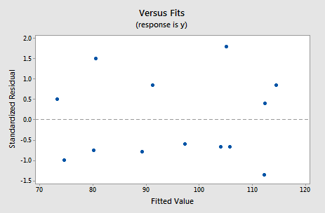
suggests that the relationship is indeed linear and that the variances of the error terms are constant. Furthermore, the normal probability plot:
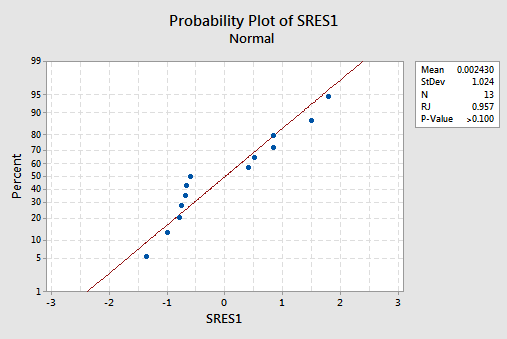
suggests that the error terms are normally distributed. The regression model with y as the response and \(x_1\) and \(x_2\) as the predictors has been evaluated fully and appears to be ready to answer the researcher's questions.
Example 10-5: IQ Size
Let's return to the brain size and body size study, in which the researchers were interested in determining whether or not a person's brain size and body size are predictive of his or her intelligence. The researchers (Willerman, et al, 1991) collected the following IQ Size data on a sample of n = 38 college students:
- Response (y): Performance IQ scores (PIQ) from the revised Wechsler Adult Intelligence Scale. This variable served as the investigator's measure of the individual's intelligence.
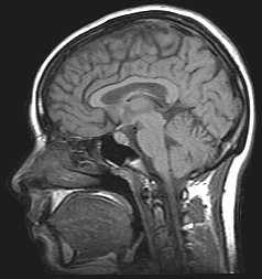
- Potential predictor (\(x_1\)): Brain size based on the count obtained from MRI scans (given as count/10,000).
- Potential predictor (\(x_2\)): Height in inches.
- Potential predictor (\(x_3\)): Weight in pounds.
A matrix plot of the resulting data looks like this:
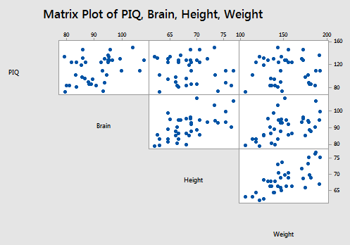
The stepwise regression procedure:
Regression analysis: PIQ versus Brain, Height, Weight
Stepwise Selection of Terms
Candidate terms: Brain, Height, Weight
| Terms | --------Step 1-------- | --------Step 2-------- | ||
|---|---|---|---|---|
| Coef | P | Coef | P | |
| Constant | 4.7 | 111.3 | ||
| Brain | 1.177 | 0.019 | 2.061 | 0.001 |
| Height | -2.730 | 0.009 | ||
| S | 21.2115 | 19.5096 | ||
| R-sq | 14.27% | 29.49% | ||
| R-sq(adj) | 11.89% | 25.46% | ||
| R-sq(pred) | 4.60% | 17.63% | ||
| Mallows' Cp | 7.34 | 2.00 | ||
\(\alpha\) to enter =0.15, \(\alpha\) to remove 0.15
yielded the final stepwise model with PIQ as the response and Brain and Height as predictors. In this case, the best subsets regression procedure:
Best Subsets Regressions: PIQ versus Brain, Height, Weight
Response is PIQ
| Vars | R-Sq | R-Sq (adj) |
R-Sq (pred) |
Mallows Cp |
S | Brain | Height | Weight |
|---|---|---|---|---|---|---|---|---|
| 1 | 2 | 3 | ||||||
| 1 | 14.3 | 11.9 | 4.66 | 7.3 | 21.212 | X | ||
| 1 | 0.9 | 0.0 | 0.0 | 13.8 | 22.810 | X | ||
| 2 | 29.5 | 25.5 | 17.6 | 2.0 | 19.510 | X | X | |
| 2 | 19.3 | 14.6 | 5.9 | 6.9 | 20.878 | X | X | |
| 3 | 29.5 | 23.3 | 12.8 | 4.0 | 19.794 | X | X | X |
yields the same model regardless of the criterion used:
- Based on the \(R^{2} \text{-value}\) criterion, the "best" model is the model with the two predictors Brain and Height.
- Based on the adjusted \(R^{2} \text{-value}\) and MSE criteria, the "best" model is the model with the two predictors of Brain and Height.
- Based on the \(C_p\) criterion, the "best" model is the model with the two predictors Brain and Height.
Well, at least, in this case, we have only one model to evaluate further:
Analysis of Variance: PIQ versus Brain, Height
| Source | DF | Adj SS | Adj MS | F-Value | P-Value |
|---|---|---|---|---|---|
| Regression | 2 | 5573 | 2786.4 | 7.32 | 0.002 |
| Brain | 1 | 5409 | 5408.8 | 14.21 | 0.001 |
| Height | 1 | 2876 | 2875.6 | 7.56 | 0.009 |
| Error | 35 | 13322 | 380.6 | ||
| Total | 37 | 18895 |
Model Summary
| S | R-sq | R-sq(adj) | R-sq(pred) |
|---|---|---|---|
| 19.5069 | 29.49% | 25.46% | 17.63% |
Coefficients
| Term | Coef | SE Coef | T-Value | P-Value | VIF |
|---|---|---|---|---|---|
| Constant | 111.3 | 55.9 | 1.99 | 0.054 | |
| Brain |
2.061 |
0.547 | 3.77 | 0.001 | 1.53 |
| Height | -2.730 | 0.993 | -2.75 | 0.009 | 1.53 |
Regression Equation
PIQ = 11.3 + 2.061 Brain - 2.730 Height
For this model, the variance inflation factors are quite satisfactory (both 1.53), the adjusted \(R^{2} \text{-value}\) (25.46%) is not great but can't get any better with these data, and the residual analysis yields no concerns. That is, the residuals versus fits plot:
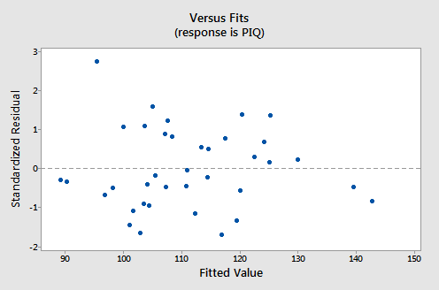
suggests that the relationship is indeed linear and that the variances of the error terms are constant. The researcher might want to investigate the one outlier, however. The normal probability plot:
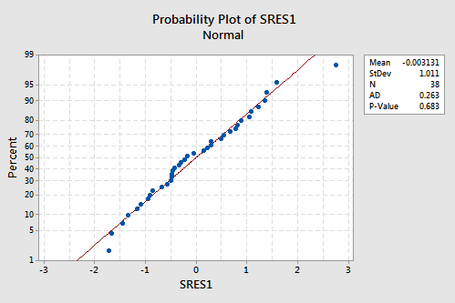
suggests that the error terms are normally distributed. The regression model with PIQ as the response and Brain and Height as the predictors has been evaluated fully and appears to be ready to answer the researchers' questions.
Example 10-6: Blood Pressure

Let's return to the blood pressure study in which we observed the following data (Blood Pressure data) on 20 individuals with hypertension:
- blood pressure (y = BP, in mm Hg)
- age (\(x_1\) = Age, in years)
- weight (\(x_2\) = Weight, in kg)
- body surface area (\(x_3\) = BSA, in sq m)
- duration of hypertension (\(x_4\) = Dur, in years)
- basal pulse (\(x_5\) = Pulse, in beats per minute)
- stress index (\(x_6\) = Stress)
The researchers were interested in determining if a relationship exists between blood pressure and age, weight, body surface area, duration, pulse rate and/or stress level.
The matrix plot of BP, Age, Weight, and BSA looks like this:
and the matrix plot of BP, Dur, Pulse, and Stress looks like this:
The stepwise regression procedure:
Regressions Analysis: BP versus Age, Weight, BSA, Dur, Pulse, Stress
Stepwise Selection of Terms
Candidate terms: x1, x2, x3, x4
| Terms | -----Step 1----- | -----Step 2----- | -----Step 3----- | |||
|---|---|---|---|---|---|---|
| Coef | P | Coef | P | Coef | P | |
| Constant | 2.21 | -16.58 | -13.67 | |||
| Weight | 1.2009 | 0.000 | 1.0330 | 0.000 | 0.9058 | 0.000 |
| Age | 0.7083 | 0.000 | 0.7016 | 0.000 | ||
| BSA | 4.63 | 0.008 | ||||
| S | 1.74050 | 0.532692 | 0.437046 | |||
| R-sq | 90.26% | 99.14% | 99.455 | |||
| R-sq(adj) | 89.72% | 99.045 | 99.35% | |||
| R-sq(pred) | 88.53% | 98.89% | 99.22% | |||
| Mallows' Cp | 312.81 | 15.09 | 6.43 | |||
\(\alpha\) to enter =0.15, \(\alpha\) to remove 0.15
yielded the final stepwise model with PIQ as the response and Age, Weight, and BSA (body surface area) as predictors. The best subsets regression procedure:
Best Subsets Regressions: BP versus Age, Weight, BSA, Dur, Pulse, Stress
Response is BP
| Vars | R-Sq | R-Sq (adj) |
R-Sq (pred) |
Mallows Cp |
S | Age | Weight | BSA | Dur | Pulse | Stress |
|---|---|---|---|---|---|---|---|---|---|---|---|
| 1 | 90.3 | 89.7 | 88.5 | 312.8 | 1.7405 | X | |||||
| 1 | 75.0 | 73.6 | 69.5 | 829.1 | 2.7903 | X | |||||
| 2 | 99.1 | 99.0 | 98.9 | 15.1 | 0.53269 | X | X | ||||
| 2 | 92.0 | 91.0 | 89.3 | 256.6 | 1.6246 | X | X | ||||
| 3 | 99.5 | 99.4 | 99.2 | 6.4 | 0.43705 | X | X | X | |||
| 3 | 99.2 | 99.1 | 98.8 | 14.1 | 0.52012 | X | X | X | |||
| 4 | 99.5 | 99.4 | 99.2 | 6.4 | 0.42591 | X | X | X | X | ||
| 4 | 99.5 | 99.4 | 99.1 | 7.1 | 0.43500 | X | X | X | X | ||
| 5 | 99.6 | 99.4 | 99.1 | 7.0 | 0.42142 | X | X | X | X | X | |
| 5 | 99.5 | 99.4 | 99.2 | 7.7 | 0.43078 | X | X | X | X | X | |
| 6 | 99.6 | 99.4 | 99.1 | 7.0 | 0.40723 | X | X | X | X | X | X |
yields various models depending on the different criteria:
- Based on the \(R^{2} \text{-value}\) criterion, the "best" model is the model with the two predictors Age and Weight.
- Based on the adjusted \(R^{2} \text{-value}\) and MSE criteria, the "best" model is the model with all six of the predictors — Age, Weight, BSA, Duration, Pulse, and Stress — in the model. However, one could easily argue that any number of sub-models are also satisfactory based on these criteria — such as the model containing Age, Weight, BSA, and Duration.
- Based on the \(C_p\) criterion, a couple of models stand out — namely the model containing Age, Weight, and BSA; and the model containing Age, Weight, BSA, and Duration.
Incidentally, did you notice how large some of the \(C_p\) values are for some of the models? Those are the models that you should be concerned about exhibiting substantial bias. Don't worry too much about \(C_p\) values that are only slightly larger than p.
Here's a case in which I might argue for thinking practically over thinking statistically. There appears to be nothing substantially wrong with the two-predictor model containing Age and Weight:
Analysis of Variance: BP versus Age, Weight
| Source | DF | Adj SS | Adj MS | F-Value | P-Value |
|---|---|---|---|---|---|
| Regression | 2 | 55.176 | 277.588 | 978.25 | 0.000 |
| Age | 1 | 49.704 | 49.704 | 175.16 | 0.000 |
| Weight | 1 | 311.910 | 311.910 | 1099.20 | 0.000 |
| Error | 17 | 4.824 | 0.284 | ||
| Lack-of-Fit | 16 | 4.324 | 0.270 | 0.54 | 0.807 |
| Pure Error | 1 | 0.500 | 0.500 | ||
| Total | 19 | 590.000 |
Model Summary
| S | R-sq | R-sq(adj) | R-sq(pred) |
|---|---|---|---|
| 0.532692 | 99.14% | 99.04% | 98.89% |
Coefficients
| Term | Coef | SE Coef | T-Value | P-Value | VIF |
|---|---|---|---|---|---|
| Constant | -16.58 | 3.01 | -5.51 | 0.000 | |
| Age |
0.7083 |
0.0535 | 13.23 | 0.000 | 1.20 |
| Weight | 1.0330 | 0.0312 | 33.15 | 0.000 | 1.20 |
Regression Equation
BP = -16.58 + 0.7083 Age + 1.0330 Weight
For this model, the variance inflation factors are quite satisfactory (both 1.20), the adjusted \(R^{2} \text{-value}\) (99.04%) can't get much better, and the residual analysis yields no concerns. That is, the residuals versus fits plot:
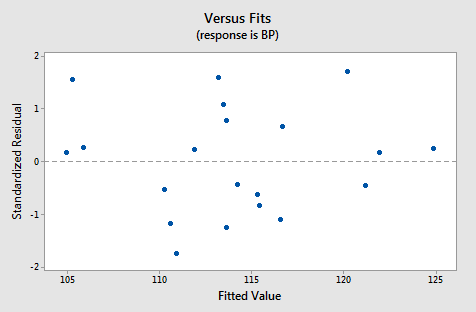
is just right, suggesting that the relationship is indeed linear and that the variances of the error terms are constant. The normal probability plot:
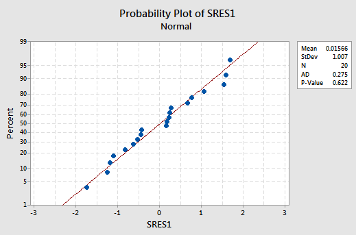
suggests that the error terms are normally distributed.
Now, why might I prefer this model over the other legitimate contenders? It all comes down to simplicity! What's your age? What's your weight? Perhaps more than 90% of you know the answer to those two simple questions. But, now what is your body surface area? And, how long have you had hypertension? Answers to these last two questions are almost certainly less immediate for most (all?) people. Now, the researchers might have good arguments for why we should instead use the larger, more complex models. If that's the case, fine. But, if not, it is almost always best to go with the simpler model. And, certainly, the model containing only Age and Weight is simpler than the other viable models.
The following video will walk through this example in Minitab.
10.5 - Information Criteria and PRESS
10.5 - Information Criteria and PRESSTo compare regression models, some statistical software may also give values of statistics referred to as information criterion statistics. For regression models, these statistics combine information about the SSE, the number of parameters in the model, and the sample size. A low value, compared to values for other possible models, is good. Some data analysts feel that these statistics give a more realistic comparison of models than the \(C_p\) statistic because \(C_p\)tends to make models seem more different than they actually are.
Three information criteria that we present are called Akaike’s Information Criterion (AIC), the Bayesian Information Criterion (BIC) (which is sometimes called Schwartz’s Bayesian Criterion (SBC)), and Amemiya’s Prediction Criterion (APC). The respective formulas are as follows:
\(AIC_{p} = n\,\text{ln}(SSE) − n\,\text{ln}(n) + 2p \)
\(BIC_{p} = n\,\text{ln}(SSE) − n\,\text{ln}(n) + p\,\text{ln}(n)\)
\(APC_{p} =\dfrac{(n + p)}{n(n − p)}SSE\)
In the formulas, n = sample size and p = number of regression coefficients in the model being evaluated (including the intercept). Notice that the only difference between AIC and BIC is the multiplier of p, the number of parameters. Each of the information criteria is used in a similar way — in comparing two models, the model with the lower value is preferred.
The BIC places a higher penalty on the number of parameters in the model so will tend to reward more parsimonious (smaller) models. This stems from one criticism of AIC in that it tends to overfit models.
The prediction sum of squares (or PRESS) is a model validation method used to assess a model's predictive ability that can also be used to compare regression models. For a data set of size n, PRESS is calculated by omitting each observation individually and then the remaining n - 1 observations are used to calculate a regression equation which is used to predict the value of the omitted response value (which, recall, we denote by \(\hat{y}_{i(i)}\)). We then calculate the \(i^{\textrm{th}}\) PRESS residual as the difference \(y_{i}-\hat{y}_{i(i)}\). Then, the formula for PRESS is given by
\(\begin{equation*} \textrm{PRESS}=\sum_{i=1}^{n}(y_{i}-\hat{y}_{i(i)})^{2}. \end{equation*}\)
In general, the smaller the PRESS value, the better the model's predictive ability.
PRESS can also be used to calculate the predicted \(R^{2}\) (denoted by \(R^{2}_{pred}\)) which is generally more intuitive to interpret than PRESS itself. It is defined as
\(\begin{equation*} R^{2}_{pred}=1-\dfrac{\textrm{PRESS}}{\textrm{SSTO}} \end{equation*}\)
and is a helpful way to validate the predictive ability of your model without selecting another sample or splitting the data into training and validation sets in order to assess the predictive ability (see Section 10.6). Together, PRESS and \(R^{2}_{pred}\) can help prevent overfitting because both are calculated using observations not included in the model estimation. Overfitting refers to models that appear to provide a good fit for the data set at hand, but fail to provide valid predictions for new observations.
You may notice that \(R^{2}\) and \(R^{2}_{pred}\) are similar in form. While they will not be equal to each other, it is possible to have \(R^{2}\) quite high relative to \(R^{2}_{pred}\), which implies that the fitted model is overfitting the sample data. However, unlike \(R^{2}\), \(R^{2}_{pred}\) ranges from values below 0 to 1. \(R^{2}_{pred}<0\) occurs when the underlying PRESS gets inflated beyond the level of the SSTO. In such a case, we can simply truncate \(R^{2}_{pred}\) at 0.
Finally, if the PRESS value appears to be large, due to a few outliers, then a variation on PRESS (using the absolute value as a measure of distance) may also be calculated:
\(\begin{equation*} \textrm{PRESS}^{*}=\sum_{i=1}^{n}|y_{i}-\hat{y}_{i(i)}|, \end{equation*}\)
which also leads to
\(\begin{equation*} R^{2*}_{pred}=1-\dfrac{\textrm{PRESS}^{*}}{\textrm{SSTO}}. \end{equation*}\)
Try It!
Predicted \(R^{2}\)
The Best Subsets output for Example 10-4
Response is y
| Vars | R-Sq | R-Sq (adj) |
R-Sq (pred) |
Mallows Cp |
S | x | x | x | x |
|---|---|---|---|---|---|---|---|---|---|
| 1 | 2 | 3 | 4 | ||||||
| 1 | 67.5 | 64.5 | 56.0 | 138.7 | 8.9639 | X | |||
| 1 | 66.6 | 63.6 | 55.7 | 142.5 | 9.0771 | X | |||
| 2 | 97.9 | 97.4 | 96.5 | 2.7 | 2.4063 | X | X | ||
| 2 | 97.2 | 96.7 | 95.5 | 5.5 | 2.7343 | X | X | ||
| 3 | 98.2 | 97.6 | 96.9 | 3.0 | 2.3087 | X | X | X | |
| 3 | 98.2 | 97.6 | 96.7 | 3.0 | 2.3232 | X | X | X | |
| 4 | 98.2 | 97.4 | 95.9 | 5.0 | 2.4460 | X | X | X | X |
The highest value of R-Sq (pred) is 96.9, which occurs for the model with x1, 2, and 4. However, recall that this model exhibits substantial multicollinearity, so the simpler model with just 1 and 2, which has a value of R-Sq (pred) of 96.5, is preferable.
Best Subsets Regressions: PIQ versus Brain, Height, Weight
Response is PIQ
| Vars | R-Sq | R-Sq (adj) |
R-Sq (pred) |
Mallows Cp |
S | Brain | Height | Weight |
|---|---|---|---|---|---|---|---|---|
| 1 | 2 | 3 | ||||||
| 1 | 14.3 | 11.9 | 4.66 | 7.3 | 21.212 | X | ||
| 1 | 0.9 | 0.0 | 0.0 | 13.8 | 22.810 | X | ||
| 2 | 29.5 | 25.5 | 17.6 | 2.0 | 19.510 | X | X | |
| 2 | 19.3 | 14.6 | 5.9 | 6.9 | 20.878 | X | X | |
| 3 | 29.5 | 23.3 | 12.8 | 4.0 | 19.794 | X | X | X |
The Best Subsets output for Example 10-5
Based on R-sq pred, the best model is the one containing Brain and Height.
Best Subsets output from Example 10-6
Best Subsets Regressions: BP versus Age, Weight, BSA, Dur, Pulse, Stress
Response is BP
| Vars | R-Sq | R-Sq (adj) |
R-Sq (pred) |
Mallows Cp |
S | Age | Weight | BSA | Dur | Pulse | Stress |
|---|---|---|---|---|---|---|---|---|---|---|---|
| 1 | 90.3 | 89.7 | 88.5 | 312.8 | 1.7405 | X | |||||
| 1 | 75.0 | 73.6 | 69.5 | 829.1 | 2.7903 | X | |||||
| 2 | 99.1 | 99.0 | 98.9 | 15.1 | 0.53269 | X | X | ||||
| 2 | 92.0 | 91.0 | 89.3 | 256.6 | 1.6246 | X | X | ||||
| 3 | 99.5 | 99.4 | 99.2 | 6.4 | 0.43705 | X | X | X | |||
| 3 | 99.2 | 99.1 | 98.8 | 14.1 | 0.52012 | X | X | X | |||
| 4 | 99.5 | 99.4 | 99.2 | 6.4 | 0.42591 | X | X | X | X | ||
| 4 | 99.5 | 99.4 | 99.1 | 7.1 | 0.43500 | X | X | X | X | ||
| 5 | 99.6 | 99.4 | 99.1 | 7.0 | 0.42142 | X | X | X | X | X | |
| 5 | 99.5 | 99.4 | 99.2 | 7.7 | 0.43078 | X | X | X | X | X | |
| 6 | 99.6 | 99.4 | 99.1 | 7.0 | 0.40723 | X | X | X | X | X | X |
Based on R-sq pred, the best models are the ones containing Age, Weight, and BSA; Age, Weight, BSA, and Duration; and Age, Weight, BSA, Duration, and Pulse.
Minitab® – Information Criteria and PRESS
10.6 - Cross-validation
10.6 - Cross-validationHow do we know that an estimated regression model is generalizable beyond the sample data used to fit it? Ideally, we can obtain new independent data with which to validate our model. For example, we could refit the model to the new dataset to see if the various characteristics of the model (e.g., estimates regression coefficients) are consistent with the model fit to the original dataset. Alternatively, we could use the regression equation of the model fit to the original dataset to make predictions of the response variable for the new dataset. Then we can calculate the prediction errors (differences between the actual response values and the predictions) and summarize the predictive ability of the model by the mean squared prediction error (MSPE). This gives an indication of how well the model will predict the future. Sometimes the MSPE is rescaled to provide a cross-validation \(R^{2}\).
However, most of the time we cannot obtain new independent data to validate our model. An alternative is to partition the sample data into a training (or model-building) set, which we can use to develop the model, and a validation (or prediction) set, which is used to evaluate the predictive ability of the model. This is called cross-validation. Again, we can compare the model fit to the training set to the model refit to the validation set to assess consistency. Or we can calculate the MSPE for the validation set to assess the predictive ability of the model.
Another way to employ cross-validation is to use the validation set to help determine the final selected model. Suppose we have found a handful of "good" models that each provide a satisfactory fit to the training data and satisfy the model (LINE) conditions. We can calculate the MSPE for each model on the validation set. Our final selected model is the one with the smallest MSPE.
The simplest approach to cross-validation is to partition the sample observations randomly with 50% of the sample in each set. This assumes there is sufficient data to have 6-10 observations per potential predictor variable in the training set; if not, then the partition can be set to, say, 60%/40% or 70%/30%, to satisfy this constraint.
If the dataset is too small to satisfy this constraint even by adjusting the partition allocation then K-fold cross-validation can be used. This partitions the sample dataset into K parts which are (roughly) equal in size. For each part, we use the remaining K – 1 parts to estimate the model of interest (i.e., the training sample) and test the predictability of the model with the remaining part (i.e., the validation sample). We then calculate the sum of squared prediction errors and combine the K estimates of prediction error to produce a K-fold cross-validation estimate.
When K = 2, this is a simple extension of the 50%/50% partition method described above. The advantage of this method is that it is usually preferable to residual diagnostic methods and takes not much longer to compute. However, its evaluation can have high variance since evaluation may depend on which data points end up in the training sample and which end up in the test sample.
When K = n, this is called leave-one-out cross-validation. That means that n separate data sets are trained on all of the data (except one point) and then a prediction is made for that one point. The evaluation of this method is very good, but often computationally expensive. Note that the K-fold cross-validation estimate of prediction error is identical to the PRESS statistic.
10.7 - One Model Building Strategy
10.7 - One Model Building StrategyWe've talked before about the "art" of model building. Unsurprisingly, there are many approaches to model building, but here is one strategy — consisting of seven steps — that are commonly used when building a regression model.
-
The First Step
Decide on the type of model that is needed to achieve the goals of the study. In general, there are five reasons one might want to build a regression model. They are:
- For predictive reasons — that is, the model will be used to predict the response variable from a chosen set of predictors.
- For theoretical reasons — that is, the researcher wants to estimate a model based on a known theoretical relationship between the response and predictors.
- For control purposes — that is, the model will be used to control a response variable by manipulating the values of the predictor variables.
- For inferential reasons — that is, the model will be used to explore the strength of the relationships between the response and the predictors.
- For data summary reasons — that is, the model will be used merely as a way to summarize a large set of data by a single equation.
-
The Second Step
Decide which predictor variables and response variables on which to collect the data. Collect the data.
-
The Third Step
Explore the data. That is:
- On a univariate basis, check for outliers, gross data errors, and missing values.
- Study bivariate relationships to reveal other outliers, suggest possible transformations, and identify possible multicollinearities.
I can't possibly overemphasize the importance of this step. There's not a data analyst out there who hasn't made the mistake of skipping this step and later regretting it when a data point was found in error, thereby nullifying hours of work.
-
The Fourth Step
Randomly divide the data into a training set and a validation set:
- The training set, with at least 15-20 error degrees of freedom, is used to estimate the model.
- The validation set is used for cross-validation of the fitted model.
-
The Fifth Step
Using the training set, identify several candidate models:
- Use best subsets regression.
- Use stepwise regression, which of course only yields one model unless different alpha-to-remove and alpha-to-enter values are specified.
-
The Sixth Step
Select and evaluate a few "good" models:
- Select the models based on the criteria we learned, as well as the number and nature of the predictors.
- Evaluate the selected models for violation of the model conditions.
- If none of the models provide a satisfactory fit, try something else, such as collecting more data, identifying different predictors, or formulating a different type of model.
-
The Seventh (and final step)
Select the final model:
- Compare the competing models by cross-validating them against the validation data.
- The model with a smaller mean square prediction error (or larger cross-validation \(R^{2}\)) is a better predictive model.
- Consider residual plots, outliers, parsimony, relevance, and ease of measurement of predictors.
And, most of all, don't forget that there is not necessarily only one good model for a given set of data. There might be a few equally satisfactory models.
10.8 - Another Model Building Strategy
10.8 - Another Model Building StrategyHere is another strategy that outlines some basic steps for building a regression model.
-
Step 1
After establishing a research hypothesis, proceed to design an appropriate experiment or experiments. Identify variables of interest, what variable(s) will be the response, and what levels of the predictor variables you wish to cover in the study. If costs allow for it, then a pilot study may be helpful (or necessary).
-
Step 2
Collect the data and make sure to "clean" it for any bugs (e.g., entry errors). If data from many variables are recorded, then variable selection and screening should be performed.
-
Step 3
Consider the regression model to be used for studying the relationship and assess the adequacy of such a model. Oftentimes, a linear regression model will be implemented. But as these notes show, there are numerous regression models and regression strategies for dealing with different data structures. How you assess the adequacy of the fitted model will be dependent on the type of regression model that is being used as well as the corresponding assumptions. For linear regression, the following need to be checked:
- Check for normality of the residuals. This is often done through a variety of visual displays, but formal statistical testing can also be performed.
- Check for the constant variance of the residuals. Again, visual displays and formal testing can both be performed.
- Check the linearity condition using residual plots.
- After time-ordering your data (if appropriate), assess the independence of the observations. Independence is best assessed by looking at a time-ordered plot of the residuals, but other time series techniques exist for assessing the assumption of independence (this is discussed further in the optional content). Regardless, checking the assumptions of your model as well as the model’s overall adequacy is usually accomplished through residual diagnostic procedures.
-
Step 4
Look for any outlying or influential data points that may be affecting the overall fit of your current model (we'll discuss this further in Lesson 11). Care should be taken with how you handle these points as they could be legitimate in how they were measured. While the option does exist for excluding such problematic points, this should only be done after careful consideration about if such points are recorded in error or are truly not representative of the data you collected. If any corrective actions are taken in this step, then return to Step 3.
-
Step 5
Assess multicollinearity, i.e., linear relationships amongst your predictor variables (we'll discuss this further in Lesson 12). Multicollinearity issues can provide incorrect estimates as well as other issues. If you proceed to omit variables or observations which may be causing multicollinearity, then return to Step 3.
-
Step 6
Use the measures discussed in this Lesson to assess the predictability and overall goodness-of-fit of your model. If these measures turn out to be unsatisfactory, then modifications to the model may be in order (e.g., a different functional form or down-weighting certain observations). If you must take such actions, then return to Step 3 afterward.
10.9 - Further Examples
10.9 - Further ExamplesExample 10-7: Peruvian Blood Pressure Data

First, we will illustrate Minitab’s “Best Subsets” procedure and a “by hand” calculation of the information criteria from earlier. Recall from Lesson 6 that this dataset consists of variables possibly relating to blood pressures of n = 39 Peruvians who have moved from rural high-altitude areas to urban lower-altitude areas (Peru dataset). The variables in this dataset (where we have omitted the calf skinfold variable from the first time we used this example) are:
Y = systolic blood pressure
\(X_1\) = age
\(X_2\) = years in urban area
\(X_3\) = \(X_2\) /\(X_1\) = fraction of life in urban area
\(X_4\) = weight (kg)
\(X_5\) = height (mm)
\(X_6\) = chin skinfold
\(X_7\) = forearm skinfold
\(X_8\) = resting pulse rate
Again, follow Stat > Regression > Regression > Best Subsets in Minitab. The results of this procedure are presented below.
Best Subsets Regressions: Systol versus Age, Years, ...
Response is Systol
| Vars | R-Sq | R-Sq (adj) |
R-Sq (pred) |
Mallows Cp |
S | Age | Years | fraclife | Weight | Height | Chin | Forearm | Pulse |
|---|---|---|---|---|---|---|---|---|---|---|---|---|---|
| 1 | 27.2 | 25.2 | 20.7 | 30.5 | 11.338 | X | |||||||
| 1 | 7.6 | 5.1 | 0.0 | 48.1 | 12.770 | X | |||||||
| 2 | 47.3 | 44.4 | 37.6 | 14.4 | 9.7772 | X | X | ||||||
| 2 | 42.1 | 38.9 | 30.3 | 19.1 | 10.251 | X | X | ||||||
| 3 | 50.3 | 46.1 | 38.6 | 13.7 | 9.6273 | X | X | X | |||||
| 3 | 49.0 | 4.7 | 34.2 | 14.8 | 9.7509 | X | X | X | |||||
| 4 | 59.7 | 55.0 | 44.8 | 7.2 | 8.7946 | X | X | X | X | ||||
| 4 | 52.5 | 46.9 | 31.0 | 13.7 | 9.5502 | X | X | X | X | ||||
| 5 | 63.9 | 58.4 | 45.6 | 5.5 | 8.4571 | X | X | X | X | X | |||
| 5 | 63.1 | 57.6 | 44.2 | 6.1 | 8.5419 | X | X | X | X | X | |||
| 6 | 64.9 | 58.3 | 3.3 | 6.6 | 8.4663 | X | X | X | X | X | X | ||
| 6 | 64.3 | 57.6 | 44.0 | 7.1 | 8.5337 | X | X | X | X | X | X | ||
| 7 | 66.1 | 58.4 | 42.6 | 7.5 | 8.4556 | X | X | X | X | X | X | X | |
| 7 | 65.5 | 57.7 | 41.3 | 8.0 | 8.5220 | X | X | X | X | X | X | X | |
| 8 | 66.6 | 57.7 | 39.9 | 9.0 | 8.5228 | X | X | X | X | X | X | X | X |
To interpret the results, we start by noting that the lowest \(C_p\) value (= 5.5) occurs for the five-variable model that includes the variables Age, Years, fraclife, Weight, and Chin. The ”X”s to the right side of the display tell us which variables are in the model (look up to the column heading to see the variable name). The value of \(R^{2}\) for this model is 63.9% and the value of \(R^{2}_{adj}\) is 58.4%. If we look at the best six-variable model, we see only minimal changes in these values, and the value of \(S = \sqrt{MSE}\) increases. A five-variable model most likely will be sufficient. We should then use multiple regression to explore the five-variable model just identified. Note that two of these x-variables relate to how long the person has lived at the urban lower altitude.
Next, we turn our attention to calculating AIC and BIC. Here are the multiple regression results for the best five-variable model (which has \(C_p\) = 5.5) and the best four-variable model (which has \(C_p\) = 7.2).
Best 5-variable model results:
Analysis of Variance
| Source | DF | Adj SS | Adj MS | F-Value | P-Value |
|---|---|---|---|---|---|
| Regression | 5 | 4171. | 834.24 | 11.66 | 0.000 |
| Age | 1 | 782.6 | 782.65 | 10.94 | 0.002 |
| Years | 1 | 751.2 | 751.19 | 10.50 | 0.003 |
| fraclife | 1 | 1180.1 | 1180.14 | 1650 | 0.000 |
| Weight | 1 | 970.3 | 970.26 | 13.57 | 0.001 |
| Chin | 1 | 269.5 | 269.48 | 3.77 | 0.061 |
| Error | 33 | 2360.2 | 71.52 | ||
| Total | 38 | 6531.4 |
Model Summary
| S | R-sq | R-sq(adj) | R-sq(pred) |
|---|---|---|---|
| 8.45707 | 63.86% | 8.39% | 45.59% |
Coefficients
| Term | Coef | SE Coef | T-Value | P-Value | VIF |
|---|---|---|---|---|---|
| Constant | 109.4 | 21.5 | 5.09 | 0.000 | |
| Age |
-1.012 |
0.306 | -3.31 | 0.002 | 2.94 |
| Years | 2.407 | 0.743 | 3.24 | 0.003 | 29.85 |
| fraclife | -110.8 | 27.3 | -4.06 | 0.000 | 20.89 |
| Weight | 1.098 | 0.298 | 3.68 | 0.001 | 2.38 |
| Chin | -1.192 | 0.614 | -1.94 | 0.061 | 1.48 |
Regression Equation
\(\widehat{Systol} = 109.4 - 1.012 Age + 2.407 Years - 110.8 fraclife + 1.098 Weight - 1.192 Chin\)
Best 4-variable model results
Analysis of Variance
| Source | DF | Adj SS | Adj MS | F-Value | P-Value |
|---|---|---|---|---|---|
| Regression | 4 | 3901.7 | 975.43 | 12.61 | 0.000 |
| Age | 1 | 698.1 | 698.07 | 9.03 | 0.005 |
| Years | 1 | 711.2 | 711.20 | 9.20 | 0.005 |
| fraclife | 1 | 1125.5 | 1125.55 | 14.55 | 0.001 |
| Weight | 1 | 706.5 | 706.54 | 9.14 | 0.005 |
| Error | 34 | 2629.7 | 77.34 | ||
| Total | 38 | 6531.4 |
Model Summary
| S | R-sq | R-sq(adj) | R-sq(pred) |
|---|---|---|---|
| 8.79456 | 59.74% | 55.00% | 44.84% |
Coefficients
| Term | Coef | SE Coef | T-Value | P-Value | VIF |
|---|---|---|---|---|---|
| Constant | 116.8 | 22.0 | 5.32 | 0.000 | |
| Age |
-0.951 |
0.316 | -3.00 | 0.005 | 2.91 |
| Years | 2.339 | 0.771 | 3.03 | 0.005 | 29.79 |
| fraclife | -108.1 | 28.3 | -3.81 | 0.001 | 20.83 |
| Weight | 0.832 | 0.275 | 3.02 | 0.005 | 1.88 |
Regression Equation
\(\widehat{Systol} = 116.8 - 0.951 Age + 2.339 Years - 108.1 fraclife + 0.832 Weight\)
AIC Comparison: The five-variable model still has a slight edge (a lower AIC is better).
- For the five-variable model:
\(AIC_p\) = 39 ln(2360.23) − 39 ln(39) + 2(6) = 172.015.
- For the four-variable model:
\(AIC_p\) = 39 ln(2629.71) − 39 ln(39) + 2(5) = 174.232.
BIC Comparison: The values are nearly the same; the five-variable model has a slightly lower value (a lower BIC is better).
- For the five-variable model:
\(BIC_p\) = 39 ln(2360.23) − 39 ln(39) + ln(39) × 6 = 181.997.
- For the four-variable model:
\(BIC_p\) = 39 ln(2629.71) − 39 ln(39) + ln(39) × 5 = 182.549.
Our decision is that the five-variable model has better values than the four-variable models, so it seems to be the winner. Interestingly, the Chin variable is not quite at the 0.05 level for significance in the five-variable model so we could consider dropping it as a predictor. But, the cost will be an increase in MSE and a 4.2% drop in \(R^{2}\). Given the closeness of the Chin value (0.061) to the 0.05 significance level and the relatively small sample size (39), we probably should keep the Chin variable in the model for prediction purposes. When we have a p-value that is only slightly higher than our significance level (by slightly higher, we mean usually no more than 0.05 above the significance level we are using), we usually say a variable is marginally significant. It is usually a good idea to keep such variables in the model, but one way or the other, you should state why you decided to keep or drop the variable.
Example 10-8: College Student Measurements

Next, we will illustrate stepwise procedures in Minitab. Recall from Lesson 6 that this dataset consists of n = 55 college students with measurements for the following seven variables (Physical dataset):
Y = height (in)
\(X_1\) = left forearm length (cm)
\(X_2\) = left foot length (cm)
\(X_3\) = left palm width
\(X_4\) = head circumference (cm)
\(X_5\) = nose length (cm)
\(X_6\) = gender, coded as 0 for male and 1 for female
Here is the output for Minitab’s stepwise procedure (Stat > Regression > Regression > Fit Regression Model, click Stepwise, select Stepwise for Method, select Include details for every step under Display the table of model selection details).
Stepwise Selection of Terms
Candidate terms: LeftArm, LeftFoot, LeftHand, headCirc, nose, Gender
| Terms | -----Step 1----- | -----Step 2----- | ||
|---|---|---|---|---|
| Coef | P | Coef | P | |
| Constant | 31.22 | 21.86 | ||
| LeftFoot | 1.449 | 0.000 | 1.023 | 0.000 |
| LeftArm | 0.796 | 0.000 | ||
| S | 2.55994 | 2.14916 | ||
| R-sq | 67.07% | 77.23% | ||
| R-sq(adj) | 66.45% | 76.35% | ||
| R-sq(pred) | 64.49% | 73.65% | ||
| Mallows' Cp | 20.69 | 0.57 | ||
\(\alpha\) to remove 0.15
All six x-variables were candidates for the final model. The procedure took two forward steps and then stopped. The variables in the model at that point are left foot length and left forearm length. The left foot length variable was selected first (in Step 1), and then the left forearm length was added to the model. The procedure stopped because no other variables could enter at a significant level. Notice that the significance level used for entering variables was 0.15. Thus, after Step 2 there were no more x-variables for which the p-value would be less than 0.15.
It is also possible to have Minitab work backward from a model with all the predictors included and only consider steps in which the least significant predictor is removed. Output for this backward elimination procedure is given below.
Backward Elimination of Terms
Candidate terms: LeftArm, LeftFoot, LeftHand, headCirc, nose, Gender
| Terms | -----Step 1----- | -----Step 2----- | -----Step 3----- | -----Step 4----- | -----Step 5----- | |||||
|---|---|---|---|---|---|---|---|---|---|---|
| Coef | P | Coef | P | Coef | P | Coef | P | Coef | P | |
| Constant | 2.1 | 19.7 | 16.60 | 21.25 | 21.86 | |||||
| LeftArm | 0.762 | 0.000 | 0.751 | 0.000 | 0.760 | 0.000 | 0.766 | 0.000 | 0.796 | 0.000 |
| LeftFoot | 0.912 | 0.000 | 0.915 | 0.000 | 0.961 | 0.000 | 1.003 | 0.000 | 1.023 | 0.000 |
| LeftHand | 0.191 | 0.510 | 0.198 | 0.490 | 0.248 | 0.332 | 0.225 | 0.370 | ||
| HeadCirc | 0.076 | 0.639 | 0.081 | 0.611 | 0.100 | 0.505 | ||||
| nose | -0.230 | 0.654 | ||||||||
| Gender | -0.55 | 0.632 | -0.43 | 0.696 | ||||||
| S | 2.20115 | 2.18317 | 2.16464 | 2.15296 | 2.14916 | |||||
| R-sq | 77.95% | 77.86% | 77.79% | 77.59% | 77.23% | |||||
| R-sq(adj) | 75.19% | 75.60% | 76.01% | 76.27% | 76.35% | |||||
| R-sq(pred) | 70.58% | 71.34% | 72.20% | 73.27% | 73.65% | |||||
| Mallows' Cp | 7.00 | 5.20 | 3.36 | 1.79 | 0.57 | |||||
\(\alpha\) to remove 0.1
The procedure took five steps (counting Step 1 as the estimation of a model with all variables included). At each subsequent step, the weakest variable is eliminated until all variables in the model are significant (at the default 0.10 level). At a particular step, you can see which variable was eliminated by the new blank spot in the display (compared to the previous step). For instance, from Step 1 to Step 2, the nose length variable was dropped (it had the highest p-value.) Then, from Step 2 to Step 3, the gender variable was dropped, and so on.
The stopping point for the backward elimination procedure gave the same model as the stepwise procedure did, with left forearm length and left foot length as the only two x-variables in the model. It will not always necessarily be the case that the two methods used here will arrive at the same model.
Finally, it is also possible to have Minitab work forwards from a base model with no predictors included and only consider steps in which the most significant predictor is added. We leave it as an exercise to see how this forward selection procedure works for this dataset (you can probably guess given the results of the Stepwise procedure above).
Software Help 10
Software Help 10
The next two pages cover the Minitab and R commands for the procedures in this lesson.
Below is a zip file that contains all the data sets used in this lesson:
- bloodpress.txt
- cement.txt
- iqsize.txt
- martian.txt
- peru.txt
- Physical.txt
Minitab Help 10: Model Building
Minitab Help 10: Model BuildingMinitab®
Martians (underspecified model)
- Perform a linear regression analysis of weight vs height + water. Click "Storage" and select "Fits" before clicking "OK."
- Select Calc > Calculator, type "FITS0" in the box labeled "Store results in variable," type "if(water=0, FITS)" in the box labeled "Expression," and click "OK." Repeat to create "FITS10" as "if(water=10,FITS)" and "FITS20" as "if(water=20,FITS)."
- Perform a linear regression analysis of weight vs height (an underspecified model). Click "Storage" and select "Fits" before clicking "OK." The resulting variable should be called "FITS_1."
- Create a basic scatterplot but select "With Groups" instead of "Simple." Plot "weight" vs "height" with "water" as the "Categorical variable for grouping."
- To add parallel regression lines representing the different levels of water to the scatterplot, select the scatterplot, select Editor > Add > Calculated Line, and select "FITS0" for the "Y column" and "height" for the "X column." Repeat to add the "FITS10" and "FITS20" lines.
- To add a regression line representing the underspecified model to the scatterplot, select the scatterplot, select Editor > Add > Calculated Line, and select "FITS_1" for the "Y column" and "height" for the "X column."
Cement hardening (variable selection using stepwise regression)
- Create a simple matrix of scatterplots of the data.
- Conduct stepwise regression for y vs \(x_1\) + \(x_2\) + \(x_3\) + \(x_4\).
IQ and body size (variable selection using stepwise regression)
- Create a simple matrix of scatterplots of the data.
- Conduct stepwise regression for PIQ vs Brain + Height + Weight.
Blood pressure (variable selection using stepwise regression)
- Create a simple matrix of scatterplots of the data.
- Conduct stepwise regression for BP vs Age + Weight + BSA + Dur + Pulse + Stress.
Cement hardening (variable selection using best subsets regression)
- Conduct best subsets regression for y vs \(x_1\) + \(x_2\) + \(x_3\) + \(x_4\).
- Perform a linear regression analysis of all four predictors (assumed unbiased) and just two predictors to retrieve the information needed to calculate \(C_p\) for the model with just two predictors by hand.
- Perform a linear regression analysis of model with \(x_1\), \(x_2\), and \(x_4\) and note the variance inflation factors for \(x_2\) and \(x_4\) are very high.
- Perform a linear regression analysis of the model with \(x_1\), \(x_2\), and \(x_3\) and note the variance inflation factors are acceptable.
- Perform a linear regression analysis of model with \(x_1\) and \(x_2\) and note the variance inflation factors are acceptable and adjusted \(R^{2}\) is high
- Create residual plots and Conduct regression error normality tests.
IQ and body size (variable selection using best subsets regression)
- Conduct best subsets regression for PIQ vs Brain + Height + Weight.
- Perform a linear regression analysis of the model with Brain and Height and note the variance inflation factors are acceptable and adjusted \(R^{2}\) is as good as it gets with this dataset.
- Create residual plots and Conduct regression error normality tests.
Blood pressure (variable selection using best subsets regression)
- Conduct best subsets regression for BP vs Age + Weight + BSA + Dur + Pulse + Stress.
- Perform a linear regression analysis of the model with Age and Weight and note the variance inflation factors are acceptable and adjusted \(R^{2}\) can't get much better.
- Create residual plots and Conduct regression error normality tests.
Peruvian blood pressure (variable selection using best subsets regression)
- Select Calc > Calculator to create fraclife variable equal to Years/Age.
- Conduct best subsets regression for Systol vs Age + Years + fraclife + Weight + Height + Chin + Forearm + Pulse.
- Perform a linear regression analysis of the best 5-predictor and 4-predictor models.
- Calculate AIC and BIC by hand.
Measurements of college students (variable selection using stepwise regression)
- Conduct stepwise regression for Height vs LeftArm + LeftFoot + LeftHand + HeadCirc + nose + Gender.
- Change the "Method" to "Backward elimination" or "Forward selection."
R Help 10: Model Building
R Help 10: Model BuildingR Help
Martians (underspecified model)
- Load the Martians data.
- Fit a multiple linear regression model of weight vs height + water.
- Fit a simple linear regression model of weight vs height.
- Create a scatterplot of weight vs height with points marked by water level and regression lines for each model.
martian <- read.table("~/path-to-data/martian.txt", header=T)
attach(martian)

model.1 <- lm(weight ~ height + water)
summary(model.1)
#              Estimate Std. Error t value Pr(>|t|)
# (Intercept) -1.220194   0.320978  -3.801  0.00421 **
# height       0.283436   0.009142  31.003 1.85e-10 ***
# water        0.111212   0.005748  19.348 1.22e-08 ***
# ---
# Residual standard error: 0.1305 on 9 degrees of freedom

model.2 <- lm(weight ~ height)
summary(model.2)
#             Estimate Std. Error t value Pr(>|t|)
# (Intercept) -4.14335    1.75340  -2.363   0.0397 *
# height       0.38893    0.04543   8.561 6.48e-06 ***
# ---
# Residual standard error: 0.808 on 10 degrees of freedom

plot(x=height, y=weight, col=water/10+1,
     panel.last = c(lines(sort(height[water==0]),
                          fitted(model.1)[water==0][order(height[water==0])],
                          col=1),
                    lines(sort(height[water==10]),
                          fitted(model.1)[water==10][order(height[water==10])],
                          col=2),
                    lines(sort(height[water==20]),
                          fitted(model.1)[water==20][order(height[water==20])],
                          col=3),
                    lines(sort(height), fitted(model.2)[order(height)], col=4)))
legend("topleft", col=1:4, pch=1, lty=1, inset=0.02,
       legend=c("Model 1, water=0", "Model 1, water=10",
                "Model 1, water=20", "Model 2"))

detach(martian)
Cement hardening (variable selection using stepwise regression)
- Load the cement data.
- Create a scatterplot matrix of the data.
- Use the
add1anddrop1functions to conduct stepwise regression.
cement <- read.table("~/path-to-data/cement.txt", header=T)
attach(cement)

pairs(cement)

model.0 <- lm(y ~ 1)
add1(model.0, ~ x1 + x2 + x3 + x4, test="F")
# Model:
# y ~ 1
#        Df Sum of Sq     RSS    AIC F value    Pr(>F)
#               2715.76 71.444
# x1      1   1450.08 1265.69 63.519 12.6025 0.0045520 **
# x2      1   1809.43  906.34 59.178 21.9606 0.0006648 ***
# x3      1    776.36 1939.40 69.067  4.4034 0.0597623 .
# x4      1   1831.90  883.87 58.852 22.7985 0.0005762 ***

model.4 <- lm(y ~ x4)
add1(model.4, ~ . + x1 + x2 + x3, test="F")
# Model:
# y ~ x4
#        Df Sum of Sq    RSS    AIC  F value    Pr(>F)
#               883.87 58.852
# x1      1    809.10  74.76 28.742 108.2239 1.105e-06 ***
# x2      1     14.99 868.88 60.629   0.1725    0.6867
# x3      1    708.13 175.74 39.853  40.2946 8.375e-05 ***

model.14 <- lm(y ~ x1 + x4)
drop1(model.14, ~ ., test="F")
# Model:
# y ~ x1 + x4
#        Df Sum of Sq     RSS    AIC F value    Pr(>F)
#                 74.76 28.742
# x1      1     809.1  883.87 58.852  108.22 1.105e-06 ***
# x4      1    1190.9 1265.69 63.519  159.30 1.815e-07 ***

add1(model.14, ~ . + x2 + x3, test="F")
# Model:
# y ~ x1 + x4
#        Df Sum of Sq    RSS    AIC F value  Pr(>F)
#               74.762 28.742
# x2      1    26.789 47.973 24.974  5.0259 0.05169 .
# x3      1    23.926 50.836 25.728  4.2358 0.06969 .

model.124 <- lm(y ~ x1 + x2 + x4)
drop1(model.124, ~ ., test="F")
# Model:
# y ~ x4 + x1 + x2
#        Df Sum of Sq    RSS    AIC  F value    Pr(>F)
#                47.97 24.974
# x1      1    820.91 868.88 60.629 154.0076 5.781e-07 ***
# x2      1     26.79  74.76 28.742   5.0259   0.05169 .
# x4      1      9.93  57.90 25.420   1.8633   0.20540

model.12 <- lm(y ~ x1 + x2)
add1(model.12, ~ . + x3 + x4, test="F")
# Model:
# y ~ x1 + x2
#        Df Sum of Sq    RSS    AIC F value Pr(>F)
#               57.904 25.420
# x3      1    9.7939 48.111 25.011  1.8321 0.2089
# x4      1    9.9318 47.973 24.974  1.8633 0.2054

detach(cement)
IQ and body size (variable selection using stepwise regression)
- Load the iqsize data.
- Create a scatterplot matrix of the data.
- Use the
add1anddrop1functions to conduct stepwise regression.
iqsize <- read.table("~/path-to-data/iqsize.txt", header=T)
attach(iqsize)

pairs(iqsize)

model.0 <- lm(PIQ ~ 1)
add1(model.0, ~ Brain + Height + Weight, test="F")
# Model:
# PIQ ~ 1
#        Df Sum of Sq   RSS    AIC F value  Pr(>F)
#               18895 237.94
# Brain   1   2697.09 16198 234.09  5.9945 0.01935 *
# Height  1    163.97 18731 239.61  0.3151 0.57802
# Weight  1      0.12 18894 239.94  0.0002 0.98806

model.1 <- lm(PIQ ~ Brain)
add1(model.1, ~ . + Height + Weight, test="F")
# Model:
# PIQ ~ Brain
#        Df Sum of Sq   RSS    AIC F value   Pr(>F)
#               16198 234.09
# Height  1   2875.65 13322 228.66  7.5551 0.009399 **
# Weight  1    940.94 15256 233.82  2.1586 0.150705

model.12 <- lm(PIQ ~ Brain + Height)
drop1(model.12, ~ ., test="F")
# Model:
# PIQ ~ Brain + Height
#        Df Sum of Sq   RSS    AIC F value    Pr(>F)
#               13322 228.66
# Brain   1    5408.8 18731 239.61 14.2103 0.0006045 ***
# Height  1    2875.6 16198 234.09  7.5551 0.0093991 **

add1(model.12, ~ . + Weight, test="F")
# Model:
# PIQ ~ Brain + Height
#        Df Sum of Sq   RSS    AIC F value Pr(>F)
#               13322 228.66
# Weight  1 0.0031633 13322 230.66       0 0.9977

detach(iqsize)
Blood pressure (variable selection using stepwise regression)
- Load the bloodpress data.
- Create scatterplot matrices of the data.
- Use the
add1anddrop1functions to conduct stepwise regression.
bloodpress <- read.table("~/path-to-data/bloodpress.txt", header=T)
attach(bloodpress)

pairs(bloodpress[,c(2:5)])
pairs(bloodpress[,c(2,6:8)])

model.0 <- lm(BP  ~ 1)
add1(model.0, ~ Age + Weight + BSA + Dur + Pulse + Stress, test="F")
# Model:
# BP ~ 1
#        Df Sum of Sq    RSS    AIC  F value    Pr(>F)
#               560.00 68.644
# Age     1    243.27 316.73 59.247  13.8248 0.0015737 **
# Weight  1    505.47  54.53 24.060 166.8591 1.528e-10 ***
# BSA     1    419.86 140.14 42.938  53.9270 8.114e-07 ***
# Dur     1     48.02 511.98 68.851   1.6883 0.2102216
# Pulse   1    291.44 268.56 55.946  19.5342 0.0003307 ***
# Stress  1     15.04 544.96 70.099   0.4969 0.4898895

model.2 <- lm(BP ~ Weight)
add1(model.2, ~ . + Age + BSA + Dur + Pulse + Stress, test="F")
# Model:
# BP ~ Weight
#        Df Sum of Sq    RSS     AIC  F value    Pr(>F)
#               54.528  24.060
# Age     1    49.704  4.824 -22.443 175.1622 2.218e-10 ***
# BSA     1     2.814 51.714  25.000   0.9251   0.34962
# Dur     1     6.095 48.433  23.689   2.1393   0.16181
# Pulse   1     8.940 45.588  22.478   3.3338   0.08549 .
# Stress  1     9.660 44.868  22.160   3.6601   0.07273 .

model.12 <- lm(BP ~ Age + Weight)
drop1(model.12, ~ ., test="F")
# Model:
# BP ~ Age + Weight
#        Df Sum of Sq    RSS     AIC F value    Pr(>F)
#                 4.82 -22.443
# Age     1    49.704  54.53  24.060  175.16 2.218e-10 ***
# Weight  1   311.910 316.73  59.247 1099.20 < 2.2e-16 ***

add1(model.12, ~ . + BSA + Dur + Pulse + Stress, test="F")
# Model:
# BP ~ Age + Weight
#        Df Sum of Sq    RSS     AIC F value   Pr(>F)
#               4.8239 -22.443
# BSA     1   1.76778 3.0561 -29.572  9.2550 0.007764 **
# Dur     1   0.17835 4.6456 -21.196  0.6143 0.444639
# Pulse   1   0.49557 4.3284 -22.611  1.8319 0.194719
# Stress  1   0.16286 4.6611 -21.130  0.5591 0.465486

model.123 <- lm(BP ~ Age + Weight + BSA)
drop1(model.123, ~ ., test="F")
# Model:
# BP ~ Age + Weight + BSA
#        Df Sum of Sq    RSS     AIC F value    Pr(>F)
#                3.056 -29.572
# Age     1    48.658 51.714  25.000 254.740 3.002e-11 ***
# Weight  1    65.303 68.359  30.581 341.886 3.198e-12 ***
# BSA     1     1.768  4.824 -22.443   9.255  0.007764 **

add1(model.123, ~ . + Dur + Pulse + Stress, test="F")
# Model:
# BP ~ Age + Weight + BSA
#        Df Sum of Sq    RSS     AIC F value Pr(>F)
#               3.0561 -29.572
# Dur     1   0.33510 2.7210 -29.894  1.8473 0.1942
# Pulse   1   0.04111 3.0150 -27.842  0.2045 0.6576
# Stress  1   0.21774 2.8384 -29.050  1.1507 0.3004

detach(bloodpress)
Cement hardening (variable selection using best subsets regression)
- Load the cement data.
- Use the
regsubsetsfunction in theleapspackage to conduct variable selection using exhaustive search (i.e., best subsets regression). Note that thenbest=2argument returns the best two models with 1, 2, ..., k predictors. - Fit models with all four predictors (assumed unbiased) and just two predictors to retrieve the information needed to calculate \(C_p\) for the model with just two predictors by hand.
- Fit model with \(x_1\), \(x_2\), and \(x_4\) and note the variance inflation factors for \(x_2\) and \(x_4\) are very high.
- Fit model with \(x_1\), \(x_2\), and \(x_3\) and note the variance inflation factors are acceptable.
- Fit model with \(x_1\) and \(x_2\) and note the variance inflation factors are acceptable, adjusted \(R^2\) is high, and a residual analysis and normality test yields no concerns.
cement <- read.table("~/path-to-data/cement.txt", header=T)
attach(cement)

library(leaps)

subset <- regsubsets(y ~ x1 + x2 + x3 + x4, method="exhaustive", nbest=2, data=cement)
cbind(summary(subset)$outmat, round(summary(subset)$adjr2, 3), round(summary(subset)$cp, 1))
#          x1  x2  x3  x4
# 1  ( 1 ) " " " " " " "*" "0.645" "138.7"
# 1  ( 2 ) " " "*" " " " " "0.636" "142.5"
# 2  ( 1 ) "*" "*" " " " " "0.974" "2.7"
# 2  ( 2 ) "*" " " " " "*" "0.967" "5.5"
# 3  ( 1 ) "*" "*" " " "*" "0.976" "3"
# 3  ( 2 ) "*" "*" "*" " " "0.976" "3"
# 4  ( 1 ) "*" "*" "*" "*" "0.974" "5"

model.1234 <- lm(y ~ x1 + x2 + x3 + x4)
model.12 <- lm(y ~ x1 + x2)

SSE.k <- sum(residuals(model.12)^2) # SSE_k = 57.90448
MSE.all <- summary(model.1234)$sigma^2 # MSE_all = 5.982955
params <- summary(model.12)$df[1] # k+1 = 3
n <- sum(summary(model.1234)$df[1:2]) # n = 13
SSE.k/MSE.all + 2*params - n # Cp = 2.678242

model.14 <- lm(y ~ x1 + x4)

SSE.k <- sum(residuals(model.14)^2) # SSE_k = 74.76211
params <- summary(model.14)$df[1] # k+1 = 3
SSE.k/MSE.all + 2*params - n # Cp = 5.495851

model.124 <- lm(y ~ x1 + x2 + x4)
library(car)
vif(model.124)
#      x1       x2       x4
# 1.06633 18.78031 18.94008

model.123 <- lm(y ~ x1 + x2 + x3)
vif(model.123)
#       x1       x2       x3
# 3.251068 1.063575 3.142125

summary(model.12)
#             Estimate Std. Error t value Pr(>|t|)
# (Intercept) 52.57735    2.28617   23.00 5.46e-10 ***
# x1           1.46831    0.12130   12.11 2.69e-07 ***
# x2           0.66225    0.04585   14.44 5.03e-08 ***
# ---
# Residual standard error: 2.406 on 10 degrees of freedom
# Multiple R-squared:  0.9787,  Adjusted R-squared:  0.9744
# F-statistic: 229.5 on 2 and 10 DF,  p-value: 4.407e-09

vif(model.12)
#       x1       x2
# 1.055129 1.055129

plot(x=fitted(model.12), y=rstandard(model.12),
     panel.last = abline(h=0, lty=2))

qqnorm(rstandard(model.12), main="", datax=TRUE)
qqline(rstandard(model.12), datax=TRUE)

library(nortest)
ad.test(rstandard(model.12)) # A = 0.6136, p-value = 0.08628

detach(cement)
IQ and body size (variable selection using best subsets regression)
- Load the iqsize data.
- Use the
regsubsetsfunction in theleapspackage to conduct variable selection using exhaustive search (i.e., best subsets regression). - Fit model with Brain and Height and note the variance inflation factors are acceptable, adjusted \(R^2\) is as good as it gets with this dataset, and a residual analysis and normality test yields no concerns.
iqsize <- read.table("~/path-to-data/iqsize.txt", header=T)
attach(iqsize)

subset <- regsubsets(PIQ ~ Brain + Height + Weight, method="exhaustive", nbest=2, data=iqsize)
cbind(summary(subset)$outmat, round(summary(subset)$adjr2, 3), round(summary(subset)$cp, 1))
#          Brain Height Weight
# 1  ( 1 ) "*"   " "    " "    "0.119"  "7.3"
# 1  ( 2 ) " "   "*"    " "    "-0.019" "13.8"
# 2  ( 1 ) "*"   "*"    " "    "0.255"  "2"
# 2  ( 2 ) "*"   " "    "*"    "0.146"  "6.9"
# 3  ( 1 ) "*"   "*"    "*"    "0.233"  "4"

model.12 <- lm(PIQ ~ Brain + Height)
summary(model.12)
#             Estimate Std. Error t value Pr(>|t|)
# (Intercept) 111.2757    55.8673   1.992 0.054243 .
# Brain         2.0606     0.5466   3.770 0.000604 ***
# Height       -2.7299     0.9932  -2.749 0.009399 **
# ---
# Residual standard error: 19.51 on 35 degrees of freedom
# Multiple R-squared:  0.2949,  Adjusted R-squared:  0.2546
# F-statistic: 7.321 on 2 and 35 DF,  p-value: 0.002208

vif(model.12)
#    Brain   Height
# 1.529463 1.529463

plot(x=fitted(model.12), y=rstandard(model.12),
     panel.last = abline(h=0, lty=2))

qqnorm(rstandard(model.12), main="", datax=TRUE)
qqline(rstandard(model.12), datax=TRUE)

ad.test(rstandard(model.12)) # A = 0.2629, p-value = 0.6829

detach(iqsize)
Blood pressure (variable selection using best subsets regression)
- Load the bloodpress data.
- Use the
regsubsetsfunction in theleapspackage to conduct variable selection using exhaustive search (i.e., best subsets regression). - Fit model with Age and Weight and note the variance inflation factors are acceptable, adjusted \(R^2\) can't get much better, and a residual analysis and normality test yields no concerns.
bloodpress <- read.table("~/path-to-data/bloodpress.txt", header=T)
attach(bloodpress)

subset <- regsubsets(BP ~ Age + Weight + BSA + Dur + Pulse + Stress,
                     method="exhaustive", nbest=2, data=bloodpress)
cbind(summary(subset)$outmat, round(summary(subset)$adjr2, 3),
      round(summary(subset)$cp, 1))
#          Age Weight BSA Dur Pulse Stress
# 1  ( 1 ) " " "*"    " " " " " "   " "    "0.897" "312.8"
# 1  ( 2 ) " " " "    "*" " " " "   " "    "0.736" "829.1"
# 2  ( 1 ) "*" "*"    " " " " " "   " "    "0.99"  "15.1"
# 2  ( 2 ) " " "*"    " " " " " "   "*"    "0.91"  "256.6"
# 3  ( 1 ) "*" "*"    "*" " " " "   " "    "0.994" "6.4"
# 3  ( 2 ) "*" "*"    " " " " "*"   " "    "0.991" "14.1"
# 4  ( 1 ) "*" "*"    "*" "*" " "   " "    "0.994" "6.4"
# 4  ( 2 ) "*" "*"    "*" " " " "   "*"    "0.994" "7.1"
# 5  ( 1 ) "*" "*"    "*" " " "*"   "*"    "0.994" "7"
# 5  ( 2 ) "*" "*"    "*" "*" "*"   " "    "0.994" "7.7"
# 6  ( 1 ) "*" "*"    "*" "*" "*"   "*"    "0.994" "7"

model.12 <- lm(BP ~ Age + Weight)
summary(model.12)
#              Estimate Std. Error t value Pr(>|t|)
# (Intercept) -16.57937    3.00746  -5.513 3.80e-05 ***
# Age           0.70825    0.05351  13.235 2.22e-10 ***
# Weight        1.03296    0.03116  33.154  < 2e-16 ***
# ---
# Residual standard error: 0.5327 on 17 degrees of freedom
# Multiple R-squared:  0.9914,  Adjusted R-squared:  0.9904
# F-statistic: 978.2 on 2 and 17 DF,  p-value: < 2.2e-16

vif(model.12)
#      Age   Weight
# 1.198945 1.198945

plot(x=fitted(model.12), y=rstandard(model.12),
     panel.last = abline(h=0, lty=2))

qqnorm(rstandard(model.12), main="", datax=TRUE)
qqline(rstandard(model.12), datax=TRUE)

ad.test(rstandard(model.12)) # A = 0.275, p-value = 0.6225

detach(bloodpress)
Peruvian blood pressure (variable selection using best subsets regression)
- Load the peru data.
- Use the
regsubsetsfunction in theleapspackage to conduct variable selection using exhaustive search (i.e., best subsets regression). - Fit the best 5-predictor and 4-predictor models.
- Calculate AIC and BIC by hand.
- Use the
stepAICfunction in theMASSpackage to conduct variable selection using a stepwise algorithm based on AIC or BIC.
peru <- read.table("~/path-to-data/peru.txt", header=T)
attach(peru)

fraclife <- Years/Age

n <- length(Systol) # 39

subset <- regsubsets(Systol ~ Age + Years + fraclife + Weight + Height + Chin +
                       Forearm + Pulse,
                     method="exhaustive", nbest=2, data=peru)
cbind(summary(subset)$outmat, round(summary(subset)$rsq, 3),
      round(summary(subset)$adjr2, 3), round(summary(subset)$cp, 1),
      round(sqrt(summary(subset)$rss/(n-c(rep(1:7,rep(2,7)),8)-1)), 4))
#          Age Years fraclife Weight Height Chin Forearm Pulse
# 1  ( 1 ) " " " "   " "      "*"    " "    " "  " "     " "   "0.272" "0.252" "30.5" "11.3376"
# 1  ( 2 ) " " " "   "*"      " "    " "    " "  " "     " "   "0.076" "0.051" "48.1" "12.7697"
# 2  ( 1 ) " " " "   "*"      "*"    " "    " "  " "     " "   "0.473" "0.444" "14.4" "9.7772"
# 2  ( 2 ) " " "*"   " "      "*"    " "    " "  " "     " "   "0.421" "0.389" "19.1" "10.2512"
# 3  ( 1 ) " " " "   "*"      "*"    " "    "*"  " "     " "   "0.503" "0.461" "13.7" "9.6273"
# 3  ( 2 ) " " "*"   "*"      "*"    " "    " "  " "     " "   "0.49"  "0.447" "14.8" "9.7509"
# 4  ( 1 ) "*" "*"   "*"      "*"    " "    " "  " "     " "   "0.597" "0.55"  "7.2"  "8.7946"
# 4  ( 2 ) "*" "*"   "*"      " "    "*"    " "  " "     " "   "0.525" "0.469" "13.7" "9.5502"
# 5  ( 1 ) "*" "*"   "*"      "*"    " "    "*"  " "     " "   "0.639" "0.584" "5.5"  "8.4571"
# 5  ( 2 ) "*" "*"   "*"      "*"    " "    " "  "*"     " "   "0.631" "0.576" "6.1"  "8.5417"
# 6  ( 1 ) "*" "*"   "*"      "*"    " "    "*"  "*"     " "   "0.649" "0.583" "6.6"  "8.4663"
# 6  ( 2 ) "*" "*"   "*"      "*"    "*"    "*"  " "     " "   "0.643" "0.576" "7.1"  "8.5337"
# 7  ( 1 ) "*" "*"   "*"      "*"    "*"    "*"  "*"     " "   "0.661" "0.584" "7.5"  "8.4556"
# 7  ( 2 ) "*" "*"   "*"      "*"    " "    "*"  "*"     "*"   "0.655" "0.577" "8"    "8.522"
# 8  ( 1 ) "*" "*"   "*"      "*"    "*"    "*"  "*"     "*"   "0.666" "0.577" "9"    "8.5228"

model.5 <- lm(Systol ~ Age + Years + fraclife + Weight + Chin)
summary(model.5)
#              Estimate Std. Error t value Pr(>|t|)
# (Intercept)  109.3590    21.4843   5.090 1.41e-05 ***
# Age           -1.0120     0.3059  -3.308 0.002277 **
# Years          2.4067     0.7426   3.241 0.002723 **
# fraclife    -110.8112    27.2795  -4.062 0.000282 ***
# Weight         1.0976     0.2980   3.683 0.000819 ***
# Chin          -1.1918     0.6140  -1.941 0.060830 .
# ---
# Residual standard error: 8.457 on 33 degrees of freedom
# Multiple R-squared:  0.6386,  Adjusted R-squared:  0.5839
# F-statistic: 11.66 on 5 and 33 DF,  p-value: 1.531e-06

k <- 5
n*log(sum(residuals(model.5)^2))-n*log(n)+2*(k+1) # AIC = 172.0151
n*log(sum(residuals(model.5)^2))-n*log(n)+log(n)*(k+1) # BIC = 181.9965

model.4 <- lm(Systol ~ Age + Years + fraclife + Weight)
summary(model.4)
#              Estimate Std. Error t value Pr(>|t|)
# (Intercept)  116.8354    21.9797   5.316 6.69e-06 ***
# Age           -0.9507     0.3164  -3.004 0.004971 **
# Years          2.3393     0.7714   3.032 0.004621 **
# fraclife    -108.0728    28.3302  -3.815 0.000549 ***
# Weight         0.8324     0.2754   3.022 0.004742 **
# ---
# Residual standard error: 8.795 on 34 degrees of freedom
# Multiple R-squared:  0.5974,  Adjusted R-squared:   0.55
# F-statistic: 12.61 on 4 and 34 DF,  p-value: 2.142e-06

k <- 4
n*log(sum(residuals(model.4)^2))-n*log(n)+2*(k+1) # AIC = 174.2316
n*log(sum(residuals(model.4)^2))-n*log(n)+log(n)*(k+1) # BIC = 182.5494

library(MASS)
subset.aic <- stepAIC(lm(Systol ~ Age + Years + fraclife + Weight + Height +
                           Chin + Forearm + Pulse), direction="both", k=2)
# Step:  AIC=172.02
# Systol ~ Age + Years + fraclife + Weight + Chin

subset.bic <- stepAIC(lm(Systol ~ Age + Years + fraclife + Weight + Height +
                           Chin + Forearm + Pulse), direction="both", k=log(n))
# Step:  AIC=182
# Systol ~ Age + Years + fraclife + Weight + Chin

detach(peru)
Measurements of college students (variable selection using stepwise regression)
- Load the Physical data.
- Use the
add1anddrop1functions to conduct stepwise regression. - Use the
regsubsetsfunction to conduct variable selection using backward elimination. - Use the
regsubsetsfunction to conduct variable selection using forward selection.
physical <- read.table("~/path-to-data/Physical.txt", header=T)
attach(physical)

gender <- ifelse(Sex=="Female",1,0)

model.0 <- lm(Height ~ 1)
add1(model.0, ~ LeftArm + LeftFoot + LeftHand + HeadCirc + nose + gender, test="F")
# Model:
# Height ~ 1
#          Df Sum of Sq     RSS    AIC  F value    Pr(>F)
#                 1054.75 164.46
# LeftArm   1    590.21  464.53 121.35  67.3396 5.252e-11 ***
# LeftFoot  1    707.42  347.33 105.36 107.9484 2.172e-14 ***
# LeftHand  1    143.59  911.15 158.41   8.3525  0.005570 **
# HeadCirc  1    189.24  865.51 155.58  11.5880  0.001272 **
# nose      1     85.25  969.49 161.82   4.6605  0.035412 *
# gender    1    533.24  521.51 127.72  54.1923 1.181e-09 ***

model.2 <- lm(Height ~ LeftFoot)
add1(model.2, ~ . + LeftArm + LeftHand + HeadCirc + nose + gender, test="F")
# Model:
# Height ~ LeftFoot
#         Df Sum of Sq    RSS     AIC F value    Pr(>F)
#                 347.33 105.361
# LeftArm   1   107.143 240.18  87.074 23.1967 1.305e-05 ***
# LeftHand  1    15.359 331.97 104.874  2.4059    0.1269
# HeadCirc  1     2.313 345.01 106.994  0.3486    0.5575
# nose      1     1.449 345.88 107.131  0.2178    0.6427
# gender    1    15.973 331.35 104.772  2.5066    0.1194

model.12 <- lm(Height ~ LeftArm + LeftFoot)
drop1(model.12, ~ ., test="F")
# Model:
# Height ~ LeftArm + LeftFoot
#          Df Sum of Sq    RSS     AIC F value    Pr(>F)
#                 240.18  87.074
# LeftArm   1    107.14 347.33 105.361  23.197 1.305e-05 ***
# LeftFoot  1    224.35 464.53 121.353  48.572 5.538e-09 ***

add1(model.12, ~ . + LeftHand + HeadCirc + nose + gender, test="F")
# Model:
# Height ~ LeftArm + LeftFoot
#          Df Sum of Sq    RSS    AIC F value Pr(>F)
#                 240.18 87.074
# LeftHand  1    3.7854 236.40 88.200  0.8167 0.3704
# HeadCirc  1    1.4016 238.78 88.752  0.2994 0.5867
# nose      1    0.4463 239.74 88.971  0.0950 0.7592
# gender    1    3.7530 236.43 88.207  0.8096 0.3725

subset <- regsubsets(Height ~ LeftArm + LeftFoot + LeftHand + HeadCirc + nose + gender,
                     method="backward", data=physical)

subset <- regsubsets(Height ~ LeftArm + LeftFoot + LeftHand + HeadCirc + nose + gender,
                     method="forward", data=physical)

detach(physical)