In this part of the lesson we will focus on model selection. Fitting all the models from the previous section to the delinquency data, we obtain the following fit statistics.
|
Model
|
X2
|
G2
|
df
|
|
Saturated
|
0.00
|
0.00
|
0
|
|
S + B
|
0.15
|
0.15
|
2
|
|
S
|
0.16
|
0.16
|
3
|
|
B
|
28.80
|
27.38
|
4
|
|
Null (intercept only)
|
36.41
|
32.96
|
5
|
The above table is an example of "analysis-of-deviance" table. This is like ANOVA table you have seen in linear regressions or similar models, where we look at the difference in the fit statistics, e.g. F-statistic, due to dropping or adding a parameter. In this case, we are checking for the change in deviance and if it is significant or not.
If a pair of models is nested (i.e. the smaller model is a special case of the larger one) then we can test
H0 : smaller model is true
versus
H1 : larger model is true
by doing likelihood ratio testing, and comparing
ΔG2 = G2 for smaller model − G2 for larger model
or
Δ X2 = X2 for smaller model − X2 for larger model
to a χ2 distribution with degrees of freedom equal to
Δdf = df for smaller model
− df for larger model.
This is exactly similar to testing whether a reduced model is true versus whether the full-model is true, for linear regression. Recall that full model has more parameters and setting some of them equal to zero the reduced model is obtained. Such models are nested, or hierarchical. The method described here holds ONLY for nested models.
For example, any model can be compared to the saturated model. The Null (intercept-only) model can be compared to any model above it. The S model or B model may be compared to S + B. But the S model cannot be directly compared to the B model because they are not nested.
The goal is to find a simple model that fits the data. For this purpose, it helps to add p-values to the analysis-of-deviance table. Here are the p-values associated with the G2 statistics:
|
Model
|
G2
|
df
|
p
|
|
Saturated
|
0.00
|
0
|
--
|
|
S + B
|
0.15
|
2
|
.928
|
|
S
|
0.16
|
3
|
.984
|
|
B
|
28.80
|
4
|
.000
|
|
Null (intercept only)
|
36.41
|
5
|
.000
|
From this table, we may conclude that:
- The Null model clearly does not fit.
- Adding B to the Null model drops the deviance by 36.41 − 28.80 = 7.61, which is highly significant because \(P(\chi^2_1 \geq 7.61)=0.006\). So the B model fits significantly better than the Null model. But the B model still is not a good fit since the goodness-of-fit chi-square value is very large.
- Adding S to the Null model drops the deviance by 36.41 − 0.16 = 36.25, and \(P(\chi^2_2 \geq 36.25)\approx 0\). So the S model fits significantly better than the Null model. And the S model fits the data very well.
- Adding B to the S model (i.e., comparing S + B to S) drops the deviance by only .01. So the fit of S + B is not significantly better than S. Both of these models fit the data well. (If S fits, then S + B must also fit, because S is a special case of S + B.) Given that both of these models fit, we prefer the S model, because it’s simpler.
Based on this table, we should choose to represent our data by the S model, because it’s the simplest one that fits the data well, thus D is conditionally independent of B given S.
But let us temporarily turn our attention to the saturated model to see how we can interpret the parameters. We can write this model as
\(\text{log}\left(\dfrac{\pi}{1-\pi}\right)=\beta_0+\beta_1 X_1+\beta_2 X_2+\beta_3 X_3+\beta_4 X_1 X_2+\beta_5 X_1 X_3\) (5)
where π is the probability of delinquency,
X1 = 1 if B = scout,
X1 = 0 otherwise
is the main effect for B, and
X2 = 1 if S = medium,
X2 = 0 otherwise,X3 = 1 if S = high,
X3 = 0 otherwise
are the main effects for S.
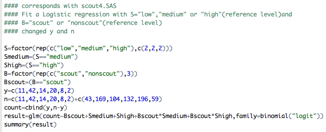
 Here is the R code in the R program scout.R that corresponds to scout4.sas:
The coefficient estimates from the output are shown below:
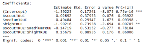
How do we interpret these effects? Referring back to equation (5),
\(\text{log}\left(\dfrac{\pi}{1-\pi}\right)=\beta_0+\beta_1 X_1+\beta_2 X_2+\beta_3 X_3+\beta_4 X_1 X_2+\beta_5 X_1 X_3\)
we see that the log-odds of delinquency for each S × B group are:
|
S
|
B
|
log-odds
|
| low | scout | β0 + β1 |
| low | non-scout | β0 |
| medium | scout | β0 + β1+ β2 + β4 |
| medium | non-scout | β0 + β2 |
| high | scout | β0 + β1+ β3 + β5 |
| high | non-scout | β0 + β3 |
Therefore,
β1 = log-odds for S = low, B = scout,
−log-odds for S = low, B = non-scout.
In other words, β1 gives the effect of scouting on delinquency when S = low. The estimate of β1 in the SAS output agrees with the B × D odds ratio for S = low,
\(\text{log}\left(\dfrac{11\times 169}{42 \times 43}\right)=0.0289\)
The effect of scouting for S = medium, however, is
β1 + β4 = log-odds for S = medium, B = scout,
−log-odds for S = medium, B = non-scout.
and the effect of scouting for S = high is
β1 + β5 = log-odds for S = high, B = scout,
−log-odds for S = high, B = non-scout.
Estimates of these latter two effects do not directly appear in the SAS or R output. How can we get them?
One way is to simply calculate them from the individual \(\hat{\beta}_j's\), and then get their standard errors from the elements of the estimated covariance matrix. For example, the estimated standard error for \(\hat{\beta}_1+\hat{\beta}_4\) is:
\(\sqrt{\hat{V}(\hat{\beta}_1)+\hat{V}(\hat{\beta}_4)+2 \hat{Cov}(\hat{\beta}_1,\hat{\beta}_4)}\)
Adding the covb option to the model statement in PROC LOGISTIC will cause SAS to print out the estimated covariance matrix. In R, one can use summary function and call the object cov.scaled (see scout.R code).
For example, since this is the saturated model we know that the odds-ratio for given the S=medium scouting level is:
\(\left(\dfrac{14/104}{20 / 132}\right)=0.8885\)
and on the log scale, log(0.8885)=-0.11827. If we read out the output from R or SAS, then \(\hat{\beta}_1+\hat{\beta}_4=0.02892-0.14719=-0.11827\) which corresponds to what we expected. To get the standard error, from the estimated covariance matrix we extract the appropriate elements, i.e.,
\(\sqrt{\hat{V}(\hat{\beta}_1)+\hat{V}(\hat{\beta}_4)+2 \hat{Cov}(\hat{\beta}_1,\hat{\beta}_4)}=\sqrt{0.14389159+0.28251130+2*(-0.14389159)}=0.3723167\)
Please note that we can certainly reduce the precision with which we are reporting these values to let's say about 4 decimal points. The values above were extracted from the R output for the estimated covariance matrix, i.e.,
> summary(result)$cov.scaled
(Intercept) BscoutTRUE SmediumTRUE ShighTRUE BscoutTRUE:SmediumTRUE BscoutTRUE:ShighTRUE
(Intercept) 0.02972668 -0.02972668 -0.02972668 -0.02972668 0.02972668 0.02972668
BscoutTRUE -0.02972668 0.14389159 0.02972668 0.02972668 -0.14389159 -0.14389159
SmediumTRUE -0.02972668 0.02972668 0.08730244 0.02972668 -0.08730244 -0.02972668
ShighTRUE -0.02972668 0.02972668 0.02972668 0.54667583 -0.02972668 -0.54667583
BscoutTRUE:SmediumTRUE 0.02972668 -0.14389159 -0.08730244 -0.02972668 0.28251130 0.14389159
BscoutTRUE:ShighTRUE 0.02972668 -0.14389159 -0.02972668 -0.54667583 0.14389159 0.79094277
Another way is to recode the model so that the estimates of interest and their standard errors appear directly in the table of coefficients. Suppose that we define the following dummy variables:
X1 = 1 if S = low, 0 otherwise
X2 = if S = low and B = scout, 0 otherwise
X3 = 1 if S = medium, 0 otherwise
X4 = 1 if S = medium and B = scout, 0 otherwise
X5 = 1 if S = high, 0 otherwise
X6 = 1 if S = high and B = scout, 0 otherwise
Then we fit the model
\(\text{log}\left(\dfrac{\pi}{1-\pi}\right)=\beta_1 X_1+\beta_2 X_2+\beta_3 X_3+\beta_4 X_4 +\beta_5 X_5+\beta_6 X_6\)
Notice that this new model does not include an intercept; an intercept would cause a collinearity problem, because X1 + X3 + X5 = 1. Under this new coding scheme, the log-odds of delinquency for each S × B group are:
|
S
|
B
|
log-odds
|
| low | scout | β1 + β2 |
| low | non-scout | β1 |
| medium | scout | β3 + β4 |
| medium | non-scout | β3 |
| high | scout | β5 + β6 |
| high | non-scout | β5 |
Therefore,
β2 = effect of scouting when S = low,
β4 = effect of scouting when S = medium,
β6 = effect of scouting when S = high.
![]() SAS code for fitting this new model is shown below (see scout.sas).
SAS code for fitting this new model is shown below (see scout.sas).
In the model statement, notice the use of the noint option to remove the intercept. The estimated table of coefficients is shown below.
 Here is the R code from the R program scout.R that corresponds to scout5.sas:
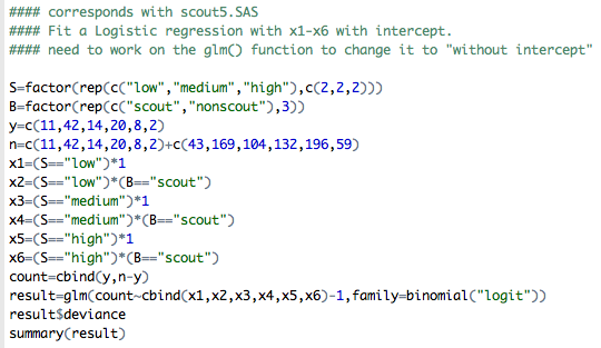
In R, you can exclude the intercept by including "-1" in the formula as seen in the code above. The estimated table of coefficients is shown below.

I will leave it to you to verify that the estimates and standard errors for β2, β4 and β6 correspond to the log-odds ratios and standard errors that we get from analyzing the B × D tables for S = low, S = medium and S = high.
These type of analysis, models and parameter interpretations extend to any k−way table. More specifically tables where we have a binary response and many other categorical variables that can have many different levels.
This is a special example of a multiple logistic regression where we have more than one explanatory variable, but they are all categorical.
Regardless of the predictor variables being categorical, continuous or a combination, when dealing with multiple predictors, model selection becomes important. With logistic regression as in ordinary multiple linear regression, we can use automated procedures such as Stepwise Procedure or Backward Elimination. These are analogous to those in ordinary multiple regression, but with a change in statistic used.
However, the more optimal procedure for logistic regression would be to use Likelihood ratio test (LRT) for testing elimination of variables, as we described with the boys scout example. If there are many categorical predictors, the sparseness can be a problem for these automated algorithms. You can also use AIC and BIC for model selection. These will be discussed along with the log-linear models later. For an example of a larger dataset, and more on Model Selection, see handouts relevant for the Water Level Study data (water.sas and water.txt):
Go to Case Studies: The Water Level Study ; or you can also see relevant files on the SAS supplemental pages (e.g., water_level1.sas, water_level2.sas). For corresponding R files see R supplemental pages (e.g., water.R)
In the next lesson we will deal with logistic regression with continuous covariates and other advanced topics.