Printer-friendly version

The chromatin in a living cell is constantly undergoing dynamic changes which enhance or inhibit transcription.  Some of these changes are mediated by proteins called transcription factors which bind to the DNA.  By chemically enhancing the binding of the protein to the DNA and then using antibodies that target a specific protein, it is possible to capture the targeted protein and its binding site.  Chromatin immunoprecipitation captures regions of the DNA that are bound the targeted protein.  DNA fragments that are not bound to the protein are washed away, leaving a sample that is enriched for the bound and tagged DNA fragments.  The protein is then released and washed away, leaving a DNA that is enriched in, but not exclusively comprised of, the fragments of interest.  

The fragments that were bound to the proteins are not identical, even if they come from the same region of DNA (in different cells) because the fragments break at different sites.  The bases bound to the protein are protected from fragmentation.  Generally the fragments include the binding site and extend beyond it.  Once the proteins are released from the proteins, they can be sequenced.  Locating the binding sites is done by mapping the sequenced fragments and determining locations on the chromosome which have more mapped reads than expected by chance.  Since fragmentation and capture is not perfectly at random, background reads are not uniformly distributed across the chromosomes, and this must be accounted for when assessing which regions have an excess of mapped reads. 

After enriching the sample for formerly bound fragments, the processing steps include:

1. Sequence the fragments.
2. Map reads to the genome.
3. Determine locations of binding sites (peaks in the distribution of mapped reads).
4. Remove artifacts due to background reads.
5. Match peak locations across samples.
6. Count reads in the peaks.
7. Differential binding analysis.

As in RNA-seq analysis, a reference is required for the mapping.  Unlike RNA-seq however, the regions of the genome corresponding to features is not known.  The features of interest are the peaks in the distribution of mapped reads.  These may vary from sample to sample and are expected to vary in intensity across treatments.  High intensity peaks are more readily found than low intensity peaks.

Both strands of DNA are bound to the proteins, and so may be captured.  The Genome Browser plot below shows the reads from the two strands in different colors.  

The red and blue instances below are mapped reads from the gata1 ChIP-seq experiment done at Penn State with red indicating one strand and blue indicating the other. 

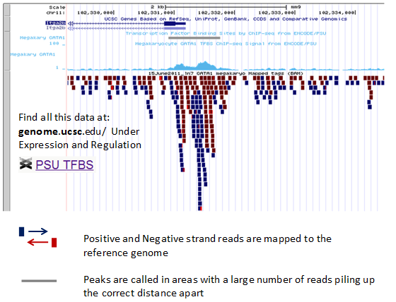
Calling Peaks

After the positive and negative strand reads are mapped to the reference genome we are ready to determine the location of the binding sites.  These are expected to produce peaks in the numbers of reads piling up at the same spot in a distinctive pattern.  Peak calling inevitably means setting some threshold for the minimum number of reads.  Pile-ups of reads that go above the threshold are called peaks. The threshold is often arbitrary and can be a point of contention in interpreting the data.  If the threshold is set too high, weak binding sites will be missed; if the threshold is set too low, random noise can be mistaken for a peak.  A statistical algorithm is used to "call" the peak locations.

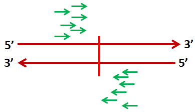
The binding sites are expected to have a distinctive double peak, due to the anti-symmetry between the properties of the two strands. We can see this in the light blue histogram above the plot. The cartoon below illustrates why the double peak occurs.  The fragments containing the binding sites are much longer than the sites themselves.  Because they are sequenced from the 5' end, the actual binding site usually beyond the sequenced part of the read.  As a result, peaks generally present a pattern of pile-ups of reads on the 5' side of the binding site.  However, generally both strands are captured, leading to symmetric pile-ups on both sides of the binding site.  This leads to a symmetric double peak with the binding site in a valley between.

There are a number of different “peak-calling methods” that can be used. The method that was used to call the peaks in our example GATA1 data is called XSET.  Each mapped read is extended to the average fragment length using the reference. This should extend the reads to include the actual binding site.  Since the reads on the two strands should form symmetric pile-ups, the number of reads at each base should form a symmetric peak as shown below.

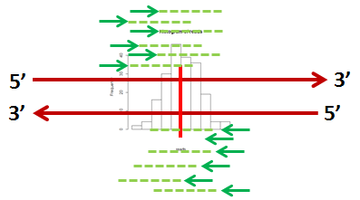
The histogram shows the number of reads at each nucleotide in the sequence.  The "peak width" is the number of bases in the peak area.  The peak intensity is the number of reads in the peak.  

However, it is not always clear where there are true peaks.  For example, there are two potential peaks below.

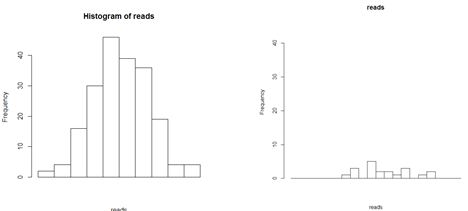
Is the histogram on the right a peak where something is binding with low binding affinity, or is this background? After locating the potential peaks, we still have to decide which ones are true peaks. This is done by thresholding and comparing to a reference sample in which there was no immunoprecitation.

Below is a visualization of reads for the GATA1 enriched sample (upper red track) and an unlabeled sample (lower red track).

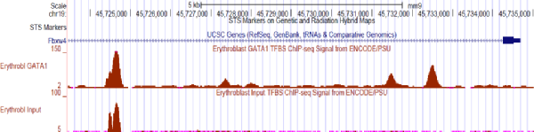
Although the first strong peak in the labeled sample seems large, the unlabeled sample also has a strong signal in that region.  This peak is potentially just background.  There are some other peaks that are fairly unambiguous.  

The most conservative thing you can do with the background is to simply mask the area and assume any reads in this area are due to background. However, you do risk missing pertinent information.  Alternatively, you can subtract out the background.

There are several peak calling programs available, and each will "call" a slightly different set of peaks if the data are at all ambiguous.  It is useful to use the Genome Browser to visualize some of the data to understand the raw read counts and where peaks have been inferred.