Printer-friendly version

Systematic and Noise Models

Statisticians often think of data as having a systematic component and a noise component.  Lets assume for now that the data Y is the log2(expression) of a particular gene (in some unspecified units).  Then a commonly used and very useful model is 

\[Y=\mu +\epsilon\]

where \(\mu\) is the systematic piece, the population mean, also written E(Y).  This is an unknown constant.

The other piece is \(\epsilon\), which is the random error or the noise. It may not be error in the colloquial sense, even though we call it \(\epsilon\) for error. It is more a mixture of measurement error and biological variation.

Straight Lines and Linear Models

For example, suppose the population is all undergraduate students at Penn State enrolled in Sept. of the current year (which is a large, but finite population).  This population has a mean weight \(\mu\) which can be determined by measuring the weight of each student and averaging.  The weight Y of an student has a deviation \(\epsilon= Y-\mu\). Even if we could perfectly measure the weights, biological variability among the students ensure that \(\epsilon\) has a distribution, often called the "error" distribution.  Because of the way that \(\epsilon\) was computed, we know that the mean of the error distribution is 0.

Now we know that weight varies with height, so we could consider the distribution of weights for students of a particular height.  For example, here is a histogram of weight versus height for Stat 200 students in 1995 (not a random sample of Penn State students):

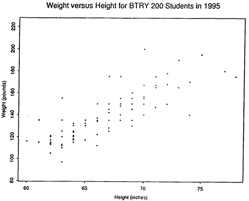
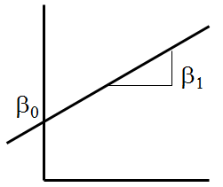
We see that the relationship between height and weight is approximately linear.  Recall that \(Z=\beta_0+\beta_1 X\) is the equation of a line with intercept \(\beta_0\) and slope \(\beta_1\). 

To take advantage of this, we might model weight as:

\[ Y=\beta_0+\beta_1 X+\epsilon\]

where

Y=weight

X=height

 If we assume that for each fixed value of X, the errors have mean zero, then the mean of Y for fixed X (written E(Y|X) or \(\mu(X)\) )is \(\beta_0+\beta_1 X\).

Now suppose we have measured n students, obtaining \(x_i,y_i\) for i=1...n.  Let

x be the column vector with entries the n values of height

y be the column vector with entries the n values of weight

\(\epsilon\) be the column vector with entries \(\epsilon_i=y_i-\beta_0+\beta_1 x_i\)

\(\beta\) be the column vector with the 2 entries \(\beta_0\) and \(\beta_1\).

and 1 be a column vector with n entries, each of which is the number "1".

Finally, let X be the matrix with columns 1 and x.

Notice that X\(\beta\) is a column vector with entries \(\beta_0+\beta_1 x_i\).

So we can write y=X\(\beta +\epsilon\) in matrix notation.  Also, note that E(Y|X)=X\(\beta\).

X is called the design matrix.  It is a matrix with known entries which is a function of our data x - in this case a column of 1's and the column with the \(x_i\) values.  \(\beta\) is a vector of unknown parameters.

In mathematics and statistics, a function f of a vector \(\alpha\) is said to be a linear function if \(f(\alpha)=M\alpha\) for some known matrix M.  In statistics, we have a linear model when E(Y|X)=M(X)\(\beta\). That is, a linear model in statistics includes the case when E(Y|X) is a straight line, but also includes other cases in which M(X) is a known matrix which is a function of X.  Note that we are using "X" in three different ways: "x" is the vector of x-variables recorded on each of our samples, "X" is the abstract x-variable (which may be random or fixed in advance) and "X" is the design matrix.

Recall that in Chapter 6 we defined two different design matrices, one for the paired t-test and the other for the two-sample t-test.  We will now show how these two tests relate to a linear model.

Paired and Two-sample t-tests Arise from Linear Models

Suppose our data arise as paired samples.  Since we are reserving X for other purposes, we will call the measured quantities Z and Y.  In a paired t-test, we change our data to D=Z-Y and test \(\mu_Z=\mu_Y\) or equivalently, \(\mu_D=\mu_Z-\mu_Y=0\) where the first equality is due to the fact that we can exchange the order of averaging and differencing, and the second equality is the null hypothesis.

Our model for the data is

\[D=\mu_D+\epsilon=\beta_0+\epsilon\]

so that \(\beta_0=\mu_D\) and \(\beta_1=0\).

The design matrix is just the column of ones and since \(\beta_1=0\) we can let \(\beta\) be the 1-vector \(\beta=\beta_0\).  Then the \(i^{th}\) entry of X\(\beta\)  is \(\beta_0\).  In this case, the test of \(\mu_D=0\) becomes a test of \(\beta_0=0\).

Note that for our two-channel microarray study, the design matrix was a column of +/1.  This is because the data was M=log2(R)-log2(G) not Z-Y.  The plus and minus signs then yields that the \(i^{th}\) entry of X\(\beta\)  is \(\beta_0\) if M=Z-Y and  \(-\beta_0\) if M=Y-Z.

Now consider the two-sample t-test.  One way to set this up is to record (X,Y) where X is "1" if the sample comes from population 1 and "0" otherwise.  Then we want to test \(\mu_1=\mu_2\) or equivalently \(\mu_1-\mu_2=0\).  The model is 

\[Y=\beta_0+\beta_1X +\epsilon.\]

Then if the sample comes from population 1, E(Y|X)=\(\mu_1=\beta_0+\beta_1\) and if the sample comes from population 2, E(Y|X)=\(\mu_2=\beta_0\).  So  \(\beta_1=\mu_1-\mu_2=0\) and our test becomes a test of \(\beta_1=0\).

Linear Models with Larger Design Matrices

The linear model is readily extended to p predictor variables \(X_1 \cdots X_p\) with observations \(x_{i1}\cdots x_{ip}\) by

\[Y=\beta_0+\beta_1X_1 +\beta_2 X_2 + \cdots \beta_pX_p +\epsilon.\]

The design matrix then has p+1 columns: the first column is 1 and column j has entries \(x_{ij}\).

Now consider one-way ANOVA with p treatments.  Let \(X_j\) be the indicator variable which is 1 if the observation came from treatment j and 0 otherwise, for j=1...(p-1).  The design matrix then consists of a column of 1's and the p-1 indicator variables.  Notice that if the observation comes from treatment j, j<p then

\[E(Y|X_1\cdots X_{p-1})=\beta_0 + \beta_j\]

and if the observation comes from treatment p, then

\[E(Y|X_1\cdots X_{p-1}]=\beta_0\].

Letting \(\mu_j\) be the \(j^{th}\) treatment mean, this means that \(\beta_0=\mu_p\) and \(\beta_j=\mu_j-\mu_p\).

If the \(p^{th}\) treatment is the control, setting up the model this way is sensible.  We can test every treatment versus the control by testing \(\beta_j=0\).  However, often we do not have a control, or other comparisons are also of interest.  In that case, a slightly different model called the cell means model is more convenient. 

Cell Means Model

We remove the column of 1's from the design matrix, but we include an indicator for treatment p.  Now our design matrix has \(x_ij) in column jand the model is

\[E(Y|X_1 \cdots X_p)=\beta_1X_1 +\beta_2 X_2 + \cdots \beta_pX_p\].

This gives \(\beta_j=\mu_j\).  We then use another matrix, called the contrast matrix, to set up the comparisons of interest such as \(\mu_1=\mu_2\) or \(\mu_1-\mu_2=\mu_3-\mu_4\). Contrast matrices are discussed in the next section.

Two-factor Designs Using Linear Models

Now suppose we have two factors, such as normal/tumor and gender.  Suppose we include two indicator variables, \(X_1=1\) for tumor tissue and \(X_1=0\) for normal  and  \(X_2 = 0\) for the males and \(X_2 = 1\) for the females. Notice that we have 4 means, \(\mu_{TF}\), \(\mu_{TM}\), \(\mu_{NF}\) and  \(\mu_{NM}\).  Letting

\[E(Y|X_1,X_2)=\beta_0+\beta_1 x_1+\beta_2 x_2.\]

Then \(\mu_{TF}=\beta_0+\beta_1+\beta_2\), \(\mu_{TM}=\beta_0+\beta_1\), \(\mu_{NF}=\beta_0+\beta_2\) and \(\mu_{NM}=\beta_0\).  We say that the effects are additive because the effect of gender and tissue type just add up.  See the plot below.

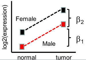
The difference in expression between normal and tumor tissue is \(\beta_1\) for both men and women .   Possibly for colon cancer this might make sense.  However, for an estrogen driven cancer the difference in expression from males to females might differ. This model does not allow for this. It only allows for a fixed difference between normal and tumor samples, (which is \(\beta_1\)), and a fixed difference between males and females, (which is \(\beta_2\)).  A more general model  allows synergy, anti-synergy or some sort of interaction between the factors.

There are several design matrices that can allow us to do this more general linear model.  One thing we could do is use the cell means model, with an indicator variable for each tissue/gender combination.  Another method is called the interaction model.  The design matrix for this model has one additional column, which is the product of \(X_1\) and \(X_2\).  Notice that \(X_1X_2=1\) only when the the sample is tumor and female.  Letting:

\[E(Y|X_1,X_2)=\beta_0+\beta_1 x_1+\beta_2 x_2+\beta_3 x_1 x_2\]

Then \(\mu_{TF}=\beta_0+\beta_1+\beta_2+\beta_3\), \(\mu_{TM}=\beta_0+\beta_1\), \(\mu_{NF}=\beta_0+\beta_2\) and\(\mu_{NM}=\beta_0\). And \(\mu_{TF}-\mu_{NF}=\beta_1+\beta_3\) while \(\mu_{TM}-\mu_{NM}=\beta_1\) so the difference between normal and tumor tissue can differ in men and women, as in the plot below.

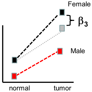
\(\beta_3\) is called the interaction between \(X_1\) and \(X_2\). \(\beta_3=(\mu_{TF}-\mu_{NF})-(\mu_{TM}-\mu_{NM})=(\mu_{TF}-\mu_{TM})-(\mu_{NF}-\mu_{NM})\) so the interaction can be described as the difference in differential expression in normal and tumor tissue for men compared to women, or the difference in differential expression in men and women for normal versus tumor tissue.

A More Complicated Experiment

What should we do if we want to include two stages or two different types of the cancer, as well as the normal samples? How would we handle this?

Another 0, 1 indicator could be put into place.

\(X_1 =1\) if the cancer is stage 1 (0 otherwise)
\(X_2 =1\) if the cancer is stage 2 (0 otherwise)

What about interaction? A tissue sample can come from a female and be either normal or tumor.  However, a sampe cannot be both stage 1 and stage 2 cancer.  So there cannot be interaction between \(X_1\) and \(X_2\) in this case (i.e. there are no samples for which \(X_1X_2=1\) ). 

Everything that we want to consider concerning gene expression should have a term in the model. We can include indicator variables for groups or variables where the ordering doesn't make sense.  We might also have continuous variables that give us linear effects, or we might have polynomial variables that give us curved effects. For instance, some responses we expect to go up with age and so we put in age without an indicator variable which would give us linear effect for age.  If there is a cyclic effect, such as cell cycles, we could put in a sine wave over time.

ANOVA and ANCOVA can also be written with linear models.