Printer-friendly version

 When all the samples are independent, differential expression can be tested using a two-sample t-test.  When all the samples are paired, differential expression can be tested using a paired t-test.  But when we have both paired and unpaired samples, use of a linear model that models both the difference in means and the shared noise components allows us to correctly incorporate all of the data into our statistical model.

A Model for the Colon Cancer Data

We have 62 tissue samples coming 40 patients.  18 patients contributed only a tumor sample, while 22 contributed both tumor and normal samples.

The systematic part of the model is the tissue type - either tumor or normal.  We set up an indicator variable X=0 for normal samples and X=1 for tumor samples.

The shared noise in the samples comes from the subject (patient).  We model this using \(b_i\) the subject "noise".  Every subject has a value of \(b_i\) even if they contributed only one sample. In this study, \(b_i\) is considered to be a block effect because the two samples from the same patient are not technical replicates - they have different values of the "treatment" which is the tissue type.

The final component is the technical noise.  This is always present in our model.  So, for every gene, our model for log2(expression) for sample j from patient i is:

\[Y_{ij}=\beta_0+\beta_1X_{ij}+b_i+\eta_{ij}\]

In a normal samples X = 0 so the gene expression is:

\[Y=\beta_0+b_i+\eta_{ij}\]

And in a tumor sample the gene expression is:

\[Y=\beta_0+\beta_1+b_i+\eta_{ij}\]

So, the difference between the two systematic pieces is \(\beta_1\). This is followed by subject noise and sample noise.

Now we have a model for the systematic tumor effects versus normal and the subject effects. In some cases there are two samples with the same subject, and there are some cases where there is only one. When we submit the model and the data to the software, the estimates of the coefficients and their SEs will be appropriately adjusted to account for paired and unpaired samples.

As part of the analysis, the software estimated the intra-class correlation as discussed in Section 7.3. The estimate  is 0.47. What does this mean?  Recall that

\[\rho=\frac{\sigma^2_b}{\sigma^2_b+\sigma^2_\eta}.\]

So, the person to person variability is about the same as the noise between the samples within the same person.  So, the variability in the 2-sample t-test (using only the unpaired samples) should be about double the variability in the paired t-test. 

Now we have done 3 different t-tests on these data - paired only using the paired t-test, unpaired only using the two-sample t-test and all the data using the linear model.  The histogram of p-values is below, along with a Venn diagram showing the genes declared as statistically significant for each case. 

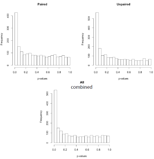
Paired samples (left), versus Paired samples (right) and all Samples Combined (below)

The combined analysis "found" 183 genes not "found" by the the paired t-test and 122 genes not "found" by the two-sample t-test, and all the genes "found" by both.   On the other hand, we might be somewhat unhappy by the discrepancies in the results!

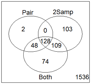
 Of these 3 analyses, I would select the linear model, which uses all the data.  That means that I would accept that 74 genes found by the combined model but not by the other methods as more likely to be true detections than the 105 genes found by the other methods but not by the combined analysis.