Printer-friendly version

We have seen how to express the population means in a t-test or ANOVA by a linear model.  We have also seen that some of the tests of interest in ANOVA can be expressed as tests of regression coefficients.  For other comparisons we will use contrasts.

What is a contrast? A contrast is essentially a difference in regression coefficients. We have seen that the regression coefficients can express a difference in means or a single mean, as well as the slope and intercept of a line. A contrast is a way of testing more general hypotheses about population means.

Suppose we have p different populations (treatments) and we have measured the expression level of the gene in a sample from each population.  The mean in population j is \(\mu_j\) and the sample mean is  \(\bar{Y}_j\).

Suppose \(c_1, c_2, … ,c_p\) are numbers and the \(\sum c_j=0\).  \(\sum c_j \mu_j\) is called a contrast of the population means.  Notice that if all the means are equal, then any contrast is zero.

We can estimate the population contrast by plugging in the sample means:

\[c_1 \bar{y}_1 +c_2 \bar{y}_2 + ... c_T \bar{y}_p \]

Notice that simple comparisons like \(\mu_1=\mu_2\) can be expressed as a contrast with \(c_1=1\) and \(c_2=-1\).  

However, contrasts can express more general comparisons.  For example, consider normal and tumor tissue in males and females with means \(\mu_{TF}\), \(\mu_{TM}\), \(\mu_{NF}\) and \(\mu_{NM}\).  We could look at the difference in gene expression in normal male and female tissue with coefficients, \(c_{TF}=c_{TM}=0\), \(c_{NF}=1\) and \(c_{NM}=-1\) (i.e. \(\mu_{NF}-\mu_{NM}=0\) ) or the difference in gene expression in males and females averaged over tissue type \(c_{TF}=c_{NF}=.5\) and \(c_{TM}=c_{NM}=-.5\)  (i.e. \(\frac{\mu_{TF}+\mu_{NF}}{2}-\frac{\mu_{TM}+\mu_{NM}}{2}=0\)). The interaction between gender and tissue type can be expressed by \(c_{TF}=c_{NM}=1\) and \(c_{TM}=c_{NF}=-1\), (i.e. \((\mu_{TF}-\mu_{NF})-\mu_{TM}-\mu_{NM})=0\)).  Any of these contrasts can be estimated by plugging in the sample means.  

To set up the model in a statistical package, you usually need to specify the factors and their interactions, as well as any blocking structure.  You do not have to set up the indicator variables.  However, you do need to figure out which contrasts you want to estimate and test, and how these are specified by the package.

If the experiment is complicated, for example if the experiment is unbalanced, has interactions, has multiple sources of noise, etc. the sample mean may not be the best estimate of the population mean.  In these cases, a better estimate of the mean can be obtained by using the maximum likelihood estimator.  Sophisticated statistical software allows you to specify the factors and error terms, and will compute appropriate estimates of the population means.    

To perform the tests is a fairly simple procedure. Statistical theory tells us that if each population is approximately Normal and has the same variance \(\sigma^2\), and the samples are independent, then if the contrast is actually 0:

\[t*=\frac{\text{Estimated Contrast}}{SE(\text{Estimated Contrast})}\]

has a t-distribution with degrees of freedom determined from the MSE.  This is just a generalization of the usual one and two-sample t-test and is based on the same statistical theory.  The MSE is computed as in ANOVA adjusted by using moderated variance estimator.  This also changes the d.f.

In complicated situations you might have to do more than one test. For example, suppose there are three populations such as three genotypes. You could set up the null hypothesis that they have identical mean expression:

\[H_0: \mu_1 = \mu_2 =\mu_3 \]

However, you can't test this with one t-test. There are different ways that this could be set up. One way would be to set up two contrasts against \(\mu_2\):

\[\mu_1 - \mu_2 =0, \;\;\; \mu_2 - \mu_3 =0 \]

Or alternatively, another common way might be:

\[\mu_1 - \mu_2 =0, \;\;\; \mu_3 - (\mu_1+\mu_2)/2 =0 \]

If all the means are equal, all 4 of these contrasts are zero.  However, if the means are not all equal, the contrasts differ in value, and so the results from the second test in each pair might vary.

 Main Effects and Interactions

If you have taken a course that covers two-way or higher ANOVA, you have likely learned about main effects and interactions.  The F-tests used to determine if these terms are statistically significantly different from zero are based on accumulating information from contrasts.  The d.f. for these terms determines the number of contrasts required.  As the simplest example, we will consider a 2-factor ANOVA with 2 levels of each factor.  For this design, the main effects and interaction all have 1 d.f., so only one contrast is required.

Lets return to our example of normal and tumor tissue in males and females.  We have already seen the contrasts for the interaction.  The contrast for the main effect of tissue type has coefficients \(c_{TF}=c_{TM}=\frac{1}{2}\), \(c_{NF}=c_{NM}=-\frac{1}{2}\) - i.e. it is the expression in tumor averaged over male and female minus the expression in normal tissue averaged over male and female.  Similarly, the contrast for the main effect of gender has coefficients \(c_{TF}=c_{NF}=\frac{1}{2}\), \(c_{TM}=c_{NM}=-\frac{1}{2}\) . The F-statistic for each effect is just the square of the t-statistic.

In general, if there are p "treatments" or factor combinations, we can express the null hypothesis of no difference in the means using p-1 linearly independent contrasts. These can be combined to form the ANOVA F-test (and is why the treatment sum of squares has p-1 d.f.)  Although the LIMMA software does compute the F-test, we usually use the tests based on the individual contrasts.  The ANOVA approach is used in MAANOVA, which is also available in Bioconductor (as well as in ANOVA and MIXED routines in SAS, SPSS, etc.).

Using the Cell Means Model

While many popular statistical packages use the main effects and interactions set-up for ANOVA, along with F-tests, the software that we will use for differential analysis makes heavy use of contrasts.  This includes the software for differential expression and differential binding (i.e. ChIP) as measured both on microarrays and sequencing platforms.  Since I find it simplest to think in terms of contrasts of the means, I prefer to use the cell means model which was discussed in Section 7.1.  The simplest way to set this up is to have an indicator variable which labels the treatment combination for each sample.  For example, suppose I have tumor/normal tissue, gender and dose 1,2,3 of a drug.  I label the treatments as TF1, TM1, ... NM3.  There are 12 different labels -- one for each of the p=12 treatments .  If I have 3 replicates, I will have a factor of length 36 with the labels for each sample in the order in which they appear in the data matrix.   

If the labels are stored in a character vector, or as a factor, then when the vector is used in a model formula, R knows to create the indicator variables for each treatment.  This makes it simple to set up the cell means model as seen in Section 7.1.  You must remember to remove the intercept, because the default in the software is to include an intercept term.

Steps in Fitting the Linear Model and Contrasts

The software we use actually has 3 steps: 

1. Set up and fit the model.
2. Set up and fit the contrasts
3. Estimate the variance using the ANOVA MSE and do the t-tests for the contrasts.

Estimating Variance

An important part of the ANOVA and regression models that we usually use is that the variance is the same in all the populations.  When this is true, a pooled estimate of the variance is an improvement on the individual sample variances.  The sample variances are the average squared deviation from the sample mean.  The pooled sample variances arise from taking the squared deviations from the sample mean and averaging over all the samples.

For example, in the plot below, each boxplot represents the samples from one treatment combination, with 4 treatments in all.  The sample means have been added to each box (blue horizontal line) and for treatment 3 the 5 observations \(Y_{31}\cdots Y_{35}\) are shown as red dots.  The residuals (also called deviations) from the sample mean are the red lines connecting the observations to the mean.  The within treatment estimate of variance is the sum of squared lengths of these lines, divided by n_i-1 where n_i is the sample size (number of biological replicates) within the treatment.  

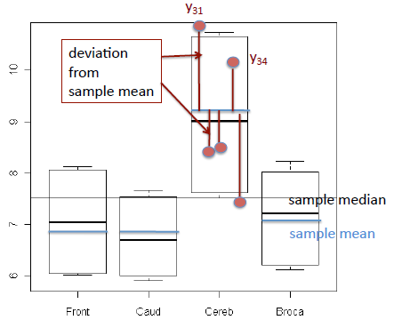
We need to have replicates in order to compute the deviations, because if there is only one observation in the treatment, then the sample mean is the same as the sample value and the deviation is zero.

The pooled estimate of the variance is the sum of the squared deviations using all the treatments, divided by the sum of the (n_i-1) which comes out to n_T - p where n_T is the total number of observations and p is the number of treatments.  This is the MSE of the ANOVA model.

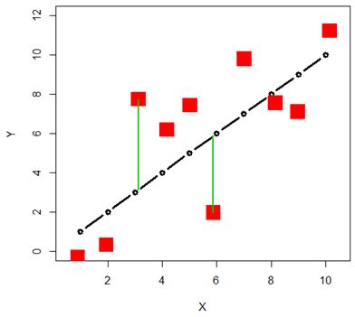
For a regression situation (for a predictor like age for instance) we do not need to have replicates for each value of the predictor. This is because the mean for each value of the predictor is estimated as the corresponding point on the line, and the deviations from the line are used in the sum of squared deviations. This is the MSE of the regression model.

Our final step in estimating the variance will be shrinkage using the empirical Bayes model as discussed in Chapter 6.