Printer-friendly version

Models for Differential Expression in Sequencing Studies

The models that we use for differential expression for RNA-seq data are extensions of the models used for microarray data.  Microarray data are intensities.  After taking log2,they are on a continuous scale and are modeled well (within gene and treatment) by the Normal distribution. Sequence data are counts. Because of this they have quite different properties than microarray data.  We need to account for the properties of count data when doing statistical analysis of RNA-seq data.

The assumption is that in unit i, there is some proportion of the reads that come from feature j. This is called \(\pi_{ij}\). We want to know whether \(\pi_{ij}\) varies systematically with the treatment, (gender, genotype, exposure or some combination these variables).

When we take a sample from unit i, we will obtain a library for sequencing with \(n_{ij}\) mapped reads from feature j. The total mapped reads in the library will be \(N_i\) and will vary among units. \(N_i\) is often referred to as the library size.  Fortunately, we always know \(N_i\) and we can account for it in our analyses.  The estimated proportion of reads from feature j will be \(p_{ij}=\frac{n_{ij}}{N_i}\), which will vary from \(\pi_{ij}\).  As well, biological replicates from the same treatment will have somewhat different values of  \(\pi_{ij}\) due to biological variability.

What we want to do is something similar to a t-test or ANOVA while taking into account that the data are counts.

Sources of Variability in Count Data

Count data have at least three sources of variability.

• Poisson variability
• biological variability
• systematic variability

Poisson variability is the variability that we would have in counts for a single gene if we took multiple technical replicates of a single RNA library and sequenced it many times. It is due to the fact that each RNA fragment either is or is not captured. There is a "Law of Small Numbers" which pretty much guarantees that when selecting a small number of fragments of a certain type in a much larger pool, as long as the fragments are selected at random and independently the number of fragments selected will have a Poisson distribution.  "A much larger pool" can generally be interpreted to mean that \(\pi_{ij}<0.01\) and \(N_i>1000\).

The Poisson distribution has a specific form that depends on \(\pi_{ij}\) and \(N_i\) for each library.  However, what affects our analysis the most is that the mean and variance of the counts for feature j from library i will both be \(N_i\pi_{ij}\).  It is this relationship between the mean count and the variation in the count that is the most important difference between continuous and count data.

How do we check the Poisson assumption? If we took one RNA sample and split this across several lanes and counted the reads for any feature in each sample, the variability that you would expect to see for that feature would be Poisson. The data we will look at in the lab has samples that were sequenced in two lanes, and we will see that the Poisson assumption fits these data very well.

As in any study in which we hope to assess biological significance, we need biological replicates of units in the same treatment.  Biological variability has to do with the fact that the \(\pi_{ij}\)'s vary among the units, even in the same treatment.  For this reason, we expect "extra Poisson variability" (this is the technical term) for counts coming from different individuals for a given feature, even if we control for the library size.

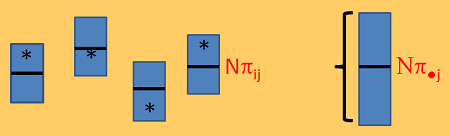
The figure below is a mock-up of the read counts you might expect from a single feature if \(N_i=N\) for every library.  The each box is a biologial replicate and indicates the data you might obtain from a sample split across several lanes.  However, typically you will obtain only one count per feature per sample, which is the asterisk in the box.  Notice that because \(N\pi_{ij}\) is about the same for all i the boxes are all about the same width.   However, when you accumulate across the biological replicates you get more variability because each sample is varying around its own \(\pi_{ij}\). This is the extra-Poisson variability.The mean proportion of reads from feature j in all possible samples from the treatment population is \(\pi_{\bullet j}\).

In order to model the data and provide appropriate tests of differential expression we will need to model the extra Poisson variability.

Differential expression analysis is meant to assess systematic variability due to the 'treatments', (genotype, exposure, tissue type, etc.) The goal is to get a p-value associated with the systematic variability. Just as with microarray data, we expression differential expression as the the ratio of estimated differences in treatment percentages, i.e. fold differences. We assess the differences in the observed fold difference relative to the total variation in the system.

Early genomics papers using sequencing data, which include SAGE tag data, often assumed that all the variability was Poisson. This means that they did not have all of the sources of the variability and it also meant that the tests used SEs that were too small yielding too many false positives.

Models that account for Extra-Poisson Variability

When all of the samples have the same library size, (which never happens),  there are two very commonly used models for the counts which account for the extra Poisson variation. The models assume that there is a probability model for the expected counts \(N_i\pi_{ij}\).

The two models both have \(n_{ij}\) distributed Poisson(\(N_i\pi_{ij}\)) with:

1) \(N_i\pi_{ij}\) ~ Gamma(a,b) which gives you Negative Binomial count data \(n_{ij}\). 

2) \(log(N_i\pi_{ij})\) ~ Normal(\(\mu_j, \sigma_j^2\)) which assumes that the log of \(N_i\pi_{ij}\) is Normal and\(n_{ij}\) is Poisson with mean \( e^{N_i\pi_{ij}}\).This is called the Poisson-LogNormal model for count data.

Most of the popular software for doing differential expression for sequence data use one of these two models with some type of adjustment to account for the fact that the library sizes are not equal.

To the left is the distribution of \(N_i\pi_{ij}\) if it is Gamma(a,b) and to the right is the distribution if it is Poisson-LogNormal

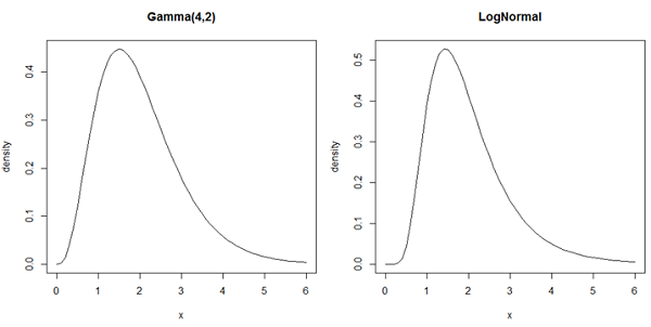
These densities are practically the same. You can see that it would be very hard to distinguish between them without extremely large sample sizes.  The software we will use assumes that the data are Negative Binomial.

Modeling the Variance of Count Data

Packages for RNA-seq differential expression analysis usually model the variance as a function of mean expression for the gene \(\mu_{ij}=N_i\pi_{\bullet j}\).  In the Negative Binomial model \(Var(n_{ij})=\mu_{ij}(1+\mu_{ij}\phi_j)\) where \(\phi_j\) is the dispersion for gene j.  When the dispersion is 0, the expression has a Poisson distribution. When \(\phi_j > 0\) then the gene has extra Poisson variation. In theory, \(\phi_j\) can also be negative but this is rarely the case.

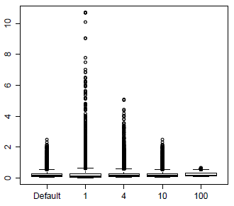
The packages vary in how they model the dispersion.  Both edgeR and DESeq2 start with a comparison of the estimated values of \(Var(n_{ij})\), estimated from the biological replicates with adjustment for the unequal library size, versus \(N_i\hat{\pi}_{\bullet j}\) where \(\hat{\pi}_{\bullet j}\) is the estimate of \(\pi_{\bullet j}\).  The default in edgeR is to plug these values in for the true variance and mean and solve for \(\phi_j\).  These values are then shrunk towards the mean dispersion, quite similarly to the variance shrinkage in LIMMA.  The amount of shrinkage is determined by a parameter called the prior d.f. which controls the relative weight of the mean dispersion versus the genewise dispersion.  The plot below shows the effects of weights prior d.f. 4, 8 and 100.  The unmoderated dispersions are very spread out, which greatly expands the y-axis of this plot and so is not shown.  The default value of 10 seems to work well in the analyses I have done.  

The effect of dispersion moderation of this type is to slightly reduce the power for testing the genes with low dispersion and to much increase the power for testing the genes with very high dispersion.  There are usually only a few of these very high dispersion genes, and they often have an unusual expression pattern with zero reads in many samples but high number of reads for biological replicates in the same treatment.  For this reason, I usually maintain a list of the high dispersion genes for a closer look.

Another option in edgeR and the default in DESeq2 is to estimate the variance by smoothing the variance for each gene against \(N_i\hat{\pi}_{ij}\) using a method similar to loess.  (Recall that we used loess to normalize 2-channel microarrays.)  Alternatively, regression models can be fitted (which is the default in edgeR when complicated log-linear models are used for modeling the log(mean) and the variance.)   In any case, the individual dispersion estimates are then shrunk toward the point on the curve, instead of to the overall mean.  

edgeR and DESeq2 use very similar models and somewhat similar dispersion shrinkage methods.  They each have their advocates.  The biggest difference is how they treat the very high dispersions.  These dispersions are shrunk the most in edgeR.  DESeq2 flags these high dispersions as outliers and does not shrink them.  As a result, these genes are often declared as discoveries by edgeR but not by DESeq2.  We will try out edgeR, but this should not be interpreted as advocating for edgeR over DESeq2.

We will also try out voom which is part of LIMMA.  voom models and shrinks the variance, rather than the dispersion.  voom does not assume that the data are Negative Binomial  - instead it uses a method called quasi-likelihood in which the regression coefficients and variance components can be estimated using weighted least squares.  edgeR and voom both come out of the Smyth lab.  Smyth seems to feel that voom is slightly better than edgeR for differential expression.  Right now, the choice among edgeR, DESeq2 and voom seems to be investigator preference.  However, there is a previous version of DESeq2 called DESeq which has lower power and should no longer be used.

Recently a students in this class tested all 4 packages with a small RNA-seq data set and considered the genes that were found to be significantly differentially expressed.  A post doctoral fellow in my lab subsequently tried all 4 packages on another data set with lots of treatments, but few replicates.  In both cases, most of the "discovered" differentially expressed genes were found by all or most of the packages.  However, both investigators found that many of the genes declared significantly differentially expressed by edgeR, DESeq or DESeq2 but not by voom had large outliers in a single sample that appeared to drive the statistical significance.  This is clearly a bad property, and so I am currently recommending voom for small datasets.  When the number of replicates is sufficiently large, it seems likely that all 4 packages will produce similar gene lists but to date I have not worked with data sets with more than a few replicates per treatment.

Linear models for the log2(expression) ,

voom uses a linear model for the data that is very similar to the usual LIMMA model.  \(Y_{ij}=log2(n_{ij})\) and

\[Y_{ij}=\beta_0+\beta_1 x_{i} +\epsilon_{ij} \]

where \(x_i\) is a variable such as an indicator for a treatment group, \(\beta_0\) and \(\beta_1\) are the slope and intercept (which are gene specific and so should depend on j).  However, unlike the usual LIMMA model, the variance of the errors, \(\epsilon_{ij}\) depends on \(N_i\pi_{\bullet j}\).

edgeR  and DESeq2 use a slightly different model called the log-linear model

\[n_{ij} \sim Negative Binomial(\mu_{ij},\phi_j)\]

where \(\mu_{ij}=N_i\pi_{\bullet j}\) and \(log2(\mu_{ij})=log2(N_i)+\beta_0+\beta_1 x_i\).

In this context, \(log2(N_i)\) is called the offset.  Since \(N_i\) the library size is known, the offset is a known constant that varies for each sample.  This is an important point in the modeling, because for normalization we do not adjust the counts, but instead we adjust the offsets using the "effective" library size.

In the linear model, the mean of \(log2(n_{ij})\) is modeled by the linear piece.  In the log-linear model, log2 of the mean of \(n_{ij}\) is modeled by the linear piece.

Except for this small difference, the model is set up in exactly the same way.  For example when I am doing ANOVA, I usually use the cell means model, with an indicator variable for each treatment and no intercept.  

Power

Recall that for a t-test, our power to detect differential expression depends on the relative size of the difference in means compared to the SE of the difference.  For count data, when there is no extra-Poisson variation, the mean and variance are the same, \(\mu_{ij}=\sigma^2_{ij}\).  This means that the ratio \(\frac{\mu_{ij}}{\sigma_{ij}}=\sqrt{\mu_{ij}}\).  The implication of this is that for a fixed fold change F in mean expression, the power to detect fold-change not equal to 1 increases when the library size increases, as well as when the number of biological replicates increase.  In sequencing studies, we therefore have more power to detect differences in more highly expressed genes.  Some downstream analyses have been developed to which take these differences into account.

We generally try to estimate the necessary sample sizes to achieve a desired power for a targeted fold change.  In sequencing studies, we might also consider the so-called sequencing depth, which can be thought of as the number of reads for the feature in the sample.  Sequencing depth can be increased by decreasing the amount of multiplexing or increasing the number of lanes on which the sample is sequenced.  Since doubling the sequencing depth for a sample costs about the same (for labeling and sequencing) as sequencing another sample, there is a trade-off that must be determined when deciding sample sizes for the study.