Printer-friendly version

Multiple Testing

Another problem with RNA-seq data has to do with multiple testing. Multiple testing adjustments all assume that if the null hypothesis is true then the p-values will be uniform. If you recall, we discussed this earlier.

This does not happen when you have count data unless you have a many, many samples or very high counts. Then things seem to average out based on the central limit theorem and look more continuous.

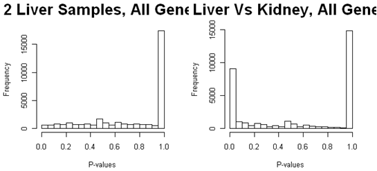
Here are the p-values from all of the genes from a study of gene expression in liver and kidney, using Fisher's exact test to compare two samples.  The weird peaks are due to the low expressing genes that have only a few possible p-values.  The peak at p=1.0 is due to the fact that no matter how many total reads there are for a feature, there is a finite probability of obtaining p=1.0 so that the p-values begin to pile up at this point - especially if there are many tests with very few reads and not much differential expression.

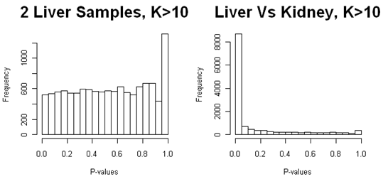
As discussed in the section on preprocessing, we should filter out (remove) genes with fewer than 10 reads in total.  Below are the p-values after we have filtered out genes that have fewer than 10 reads per feature. We still have a peak at p=1.0 (and this is really at p=1.0, not the bin from 0.95 to 1.0) for the comparison of liver samples, in which there is no differential expression. There is also a small peak at p=1.0 for the comparison of liver and kidney samples, but it is obscured because there is a lot of differential expression.  Note that with continuous data such as microarray intensity data, there should never be a peak near p=1.0, and p-values should also never be 1.0 (although it could occur due to round-off error).

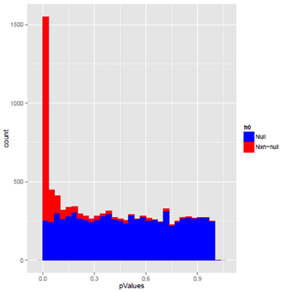
Here are some simulated data to show this again. The first plot is simulated data which mimics what you might obtain in a microarray study.The data are continuous and were analysed using a two-sample t-test.  The blue p-values came from features that were simulated to have no difference in the means, i.e. they were all null. The red were simulated to have a difference in means.

The blue p-values are not completely flat, although statistical theory states that they should be.  This is stochastic variability - the slight ups and downs will be in different places in different samples, and will flatten out if there are lots of features. Most of the red p-values are skewed towards p = 0 where they should be, as this was a test with high power. There is a thin layer of spread crossed the remaining bins, because even with high power there is some probability of a large p-value. 

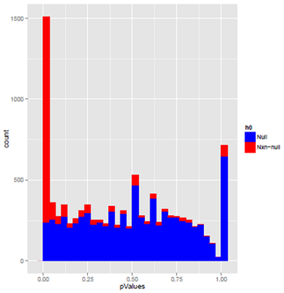
This is a similar plot for simulated RNA-seq data. The blue p-values from the features with no difference in means doesn't look the least bit uniform. Most of the peak at p=1.0 resulted from features that had two or three reads, the others came from features that have slightly more. The dip near p=1.0 is due to the fact that when there are very few total reads, there are no p-values between .9 and 1.0.  As in the microarray data, the features that were simulated to have differential expression mostly have very small p-values.  However, even when the null hypothesis is false, a fair number of the tests give p=1.0.  These mostly come from features with very few reads.

The bottom line is that multiple testing has problems if you don't throw out the the features with low counts. One reason is that there is not enough information to reject and the other is this weird shape to the histogram  of p-values.  Although there are a few papers suggesting different ways to fix the p-value histograms to use with multiple testing adjustments, work with my students strongly suggests that after filtering out the features with very few counts, the standard methods such as BH and Storey's method work fine for FDR adjustment.