Printer-friendly version

As an example of the use of SVD to detect patterns, we will consider the primate brain data from homework 5.  These data came from a microarray study of gene expression brains from 3 humans and 3 chimpanzees, dissected into 4 brain regions before RNA extraction and hybridized to Affymetrix human microarrays.  The data were normalized using RMA and we used LIMMA to compute the mean of each gene expression for each brain region.  The homework stored the mean log2(expresson) for each gene for each brain region in FitTrtMeans\$coef.

Although SVD can be used with the individual samples, when there are multiple treatments and multiple replicates per treatment, we often average the expression of each gene over the replicates before doing gene clustering or finding eigengenes.   For this example we used the 200 most significantly differentially expressed genes as determined using LIMMA and M=FitTrtMeans\$coef.

Recall that brain regions 1 -- 4 came from chimpanzees and 5 -- 8 came from humans.  Regions 1 and 5 are Broca's region, 2 and 6 are Caudate, 3 and 7 are Cerebellum and 4 and 8 are Prefrontal cortex.

Analysis using Euclidean Distance

I used complete linkage clustering with Euclidean distance to cluster the genes, and then used cutree to create 6 clusters.  The mean of the genes in each of the 4 largest clusters is shown below in the left-hand panel.  (The right panel displays the clusters obtained using correlation distance and will be discussed later.)  We can see that the most dominant pattern is differential expression between cerebellum and the other brain regions, although there is also a pattern of differential expression in caudate.  There appear to be few differences between chimpanzees and humans in these patterns.  As well, it appears that clusters 2 and 4 could be merged.

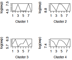
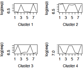
 Figure 1: Cluster profiles using Euclidean distance                           Cluster profiles using correlation distance

We now look at patterns in the data using SVD.  Our matrix M has g=200 features (genes) and n=8 treatment means (so I will call the columns of V "eigentreatments" instead of eigensamples).  Notice that this implies that there are 8 eigengenes and 8 eigentreatments.  

Here are the first four eigengenes plotted against brain regions. Again we see that cerebellum and caudate create most of the patterns.  

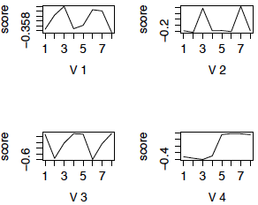
Figure 2: First 4 eigengenes using SVD

Notice that three of the the patterns are very similar to the cluster profiles, and seem to have a clear interpretation.  For example, the first 3 eigengenes are genes that are differentially expressed between specific brain regions and are expressed in the same way in chimpanzees and humans.  Eigengene 4 is the pattern of differential expression between humans and chimpanzees.  Note however, that in SVD, unlike clustering, the direction of the pattern does not matter - i.e. in eigengene 2, all the genes that are differentially expressed in regions 3 and 7 (cerebellum) compared to the other regions contribute to the eigengene, whether they are up or down

There are several main differences between the patterns one obtains from SVD compared to finding clusters and then averaging within cluster:

1) The number of clusters of features is limited only by the total number of features.  The number of clusters of samples is limited only by the total number of samples.  But in SVD, there are at most min(g,n) eigenfeatures and eigensamples.  

2) Clusters do not have an order of importance.  The eigencomponents are ordered by the singular values.  Often a the proportion of variance explained by the first few singular values is close to 1 and only the associated eigencomponents are considered important.

3) If the features and samples are clustered separated (e.g. a heatmap) there is no association between the feature clusters and the sample clusters.  However, the i^th eigensample and eigenfeature are associated through the decomposition.

4) Each pattern that is found in a cluster could be flipped horizontally, which would lead to another cluster.  However, the eigencomponents and their mirror images are the same.

Another idea that has been used (WCGNA) is to cluster first and then use SVD within clusters.  Often, however, only the first eigengene appears to be important, and it is highly correlated with the cluster mean.

Analysis using PCA with the Variance Matrix (analogous to Euclidean distance)

We now redo the SVD using the row (gene) centered data.  This is also called PCA (using the variance matrix).  The first 4 eigengenes are displayed in the left panel below.  (The right panel are the eigengenes using the z-scores of the genes, i.e. PCA using the correlation matrix, and will be discussed later.)  Notice that 3 of the 4 eigengenes are very similar to the eigengenes from the uncentered analysis (except for possible flipping to the mirror image).  However, centered eigengene 3 is something new.  Note that the scores for the chimpanzee brain regions are the flipped version of the scores for the human brain regions.  This eigengene is an interaction of species with some of the brain regions.

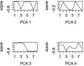
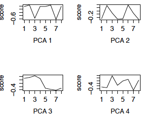
                       Figure 3:  First 4 PCs, Centered only                                                        First 4 PCs, z-scores

 Analysis using correlation distance

We now redo the analysis using the z-scores of log2(expression) for each gene.  We start by looking at the cluster profiles after using hierarchical clustering with correlation distance and cutting into 6 clusters.  We show the profiles of the 4 largest clusters in the right panel of FIgure 1.  The missing clusters have 3 and 1 genes respectively.  Again the cluster profiles appear to be based primarily on differential expression in cerebellum and caudate, with little difference between species.  They are quite similar to the cluster profiles using Euclidean distance.

The eigengenes computed from the z-scores shown in the right panel of Figure 3 are quite similar to those computed from the centered data (PCA 4 is flipped) and have similar interpretations.

Comments

In this case, the eigengenes associated with the 4 largest singular values were readily interpretable.  However, this need not always be the case.  Often, only the first eigengene is interpretable, as the subsequence eigengenes are constrained to be uncorrelated.  For example, if the two most dominant patterns in the data are correlated, then the most dominant pattern will be the first eigengene, and the second pattern will be a weighted average of the first and second eigengene.  

In the case of SVD and PCA, the idea of "dominant pattern" can be made precise through the use of the singular values (SVD) or eigenvalues (squared singular values, PCA).  This is the topic of the next section.