Printer-friendly version

SVD, PCA and Clustering

There are several ways to combine clustering with 'eigen' methods. Some methods such as WGCNA [https://horvath.genetics.ucla.edu/html/CoexpressionNetwork/Rpackages/WGCNA/] find clusters and then use eigenfeatures within each cluster. For instance, cluster analysis is performed on all of the genes without doing any filtering on it differential expression. Everything is clustered and then an SVD is done on each cluster. Often what happens is that each cluster has one dominant eigencomponent, the cluster profile. This reassure you that the cluster has been correctly identified -if there are multiple important components it is likely that the cluster should be split.

Usually the eigenfeatures are used for plotting, i.e., feature i is plotted as \((U_{i1},U_{i2})\).  This is called the plot against the first 2 principal components.  We might also plot against principal components 1 and 3, and 2 and 3 if the first two principal components do not explain most of the variance. There is also a more complicated plot called the biplot which helps you determine which gene(s) have the dominant patterns.  Biplots are not intuitive, but they are very informative once you have learned to interpret them.

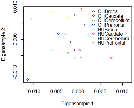
PCA is highly related to k-means clustering.  Many k-means clustering packages plot the data against the PCs to visualize the clusters, as the cluster centers are often well spread out in the eigenfeature directions. The plot of the treatment means against the first two eigentreatments for the brain data is below - no interesting clusters appear to be in these data.  The plot against the eigengenes is equally uninformative in this case.  

Denoising using SVD

Another use for SVD is for noise reduction. Unlike differential expression analysis, SVD and PCA can find patterns in unreplicated data.  After choosing the number of eigencomponents k the denoised version of M is 

\[\hat{M}=\sum_{i=1}^k U_i d_{ii} V_i^\top .\]

If we start by centering the data (PCA), we also need to add back the row mean to every row.  As mentioned earlier, this is equivalent to regressing the entries of M on the left or right singular values.  It can be shown that for any number of predictors k the SVD reconstruction of M is the linear predictor which most reduces the residual sum of squares. 

Missing value imputation using SVD

You can also use the denoised version of M to fill in any missing values by prediction. This requires an SVD algorithm such as SVDmiss in the R package SpatioTemporal  which can estimate the singular values and singular vectors with missing values.  We then replace any missing entries \(M_{ij}\) by \(\hat{M}_{ij}\).  We tend to get better prediction if we use a small number of components k  when doing the imputation, as we are then fitting the strongest patterns in the data, rather than the random components.  The SVD is one of the best ways of doing imputation of missing data.

SVD, PCA and patterns in the data matrix

The maximum number of singular vectors or principal components is the same as min(g,n) - i.e. the number of samples or features.  . This doesn't mean that we don't have more patterns in the data.  SVD and PCA find a "basis" for the patterns - i.e. every pattern in the data is a weighted average of the singular vectors.

Other pattern finding methods using matrix decomposition

There are other 'latent structure' models that use this kind of matrix decomposition. Factor analysis is very similar to singular value decomposition and principal components analysis.

Another method, called independent component analysis ICA attempts to find statistically independent components to the data matrix.  For Normally distributed data, independent is the same as uncorrelated, and this reduces to PCA.  However, for non-Normal data, ICA may find other interesting structure.

Machine learning has given us another matrix decomposition method called nonnegative matrix decomposition that decomposes M as a produce of the form

\[\hat{M}=AB^\top\]

where A is an n × k matrix and B is a k × k matrix both of which have only nonnegative entries (i.e. every number in the matrices is zero or positive).  Compared to using SVD to predict or denoise M, the resulting \(\hat{M}\) is often quite similar.  However, the entries of A (the eigensamples) and B (the eigengenes) are all nonnegative, which is compelling when the original data matrix M has only nonnegative entries since we would not want to have negative expression.  The resulting matrices may not be unique but often have properties had enhance interpretability, such as having many zero entries.

Finally, ordination methods can be used to find axes which spread out the data as much as possible.  For example, we could use the Euclidean distance as a measure of distance between samples (using our g genes) and then try to find a much smaller set of variables which give us almost the same distance matrix - these variables are called ordination axes.  They will have a co-ordinate for every sample, and so they have the dimension of eigenfeatures.  Multidimensional scaling is a popular ordination method which is sometimes referred to a nonparametric PCA.