Printer-friendly version

Principal components analysis is one of the most common methods used for linear dimension reduction. The motivation behind dimension reduction is that, the process gets unweildy with a large number of variables while the large number does not add any new information to the process. An analogy may be drawn with variance inflation factors in multiple regression. If VIF corresponding to any predictor is large, that predictor is not included in the model, as that variable does not contribute any new information. On the other hand, because of linear dependence, the regression matrix may become singular. In a multivariate situation, it may well happen that, a few (or a large number of) variables have high interdependence. A linear combination of variables is then considered which are orthogonal to one another, but the total variability within the sample is preserved as much as possible.

Suppose the data is 10-dimensional but needs to be reduced to 2-dimensional. The idea of principal component analysis is to use two directions that capture the variation in the data as much as possible. 

[Keep in mind that the dimensions to which data needs to be reduced, is usually not pre-fixed. After taking a look at the total proportion of variability captured, the reduction in dimension is determined. Here reduction of 10-dimensional space to 2-diemnsion space is for illustration only]

The sample covariance matrix of X is given as:

\[ S=\textrm{X}^T\textrm{X} /N \].

If you do the Eigen decomposition of \(X^TX\):

\[\begin{align*}\textrm{X}^T\textrm{X}
 &= (\textrm{U}\textrm{D}\textrm{V}^T)^T(\textrm{U}\textrm{D}\textrm{V}^T)\\
 &= \textrm{V}\textrm{D}^T\textrm{U}^T\textrm{U}\textrm{D}\textrm{V}^T\\
 &=\textrm{V}\textrm{D}^2\textrm{V}^T
\end{align*}\]

It turns out that if you have done the singular value decomposition then you already have the Eigen value decomposition for \(X^TX\).

The \(D^2\) is the diagonal part of matrix D with every element on the diagonal squared.

Also, we should point out that we can show using linear algebra that \(X^TX\) is a semi-positive definite matrix. This means that all of the eigenvalues are guaranteed to be nonnegative. The eigen values are in matrix \(D^2\). Since these values are squared, every diagonal element is non-negative.

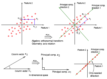
The eigenvectors of \(X^TX\), \(v_j\), can be obtained either by doing an Eigen decomposition of \(X^TX\), or by doing a singular value decomposition from X. These v_j's are called principal component directions of X. If you project X onto the principal components directions you get the principal components.

• It's easy to see that \(\mathbf{z}_j = \mathbf{X}\mathbf{v}_j = \mathbf{u}_j d_j\) . Hence \(\mathbf{u}_j\) is simply the projection of the row vectors of \(\mathbf{X}\), i.e., the input predictor vectors, on the direction \(\mathbf{v}_j\), scaled by \(d_j\). For example:

\( \textrm{z}_1=\begin{pmatrix}
X_{1,1}v_{1,1}+X_{1,2}v_{1,2}+ ... +X_{1,p}v_{1,p}\\
X_{2,1}v_{1,1}+X_{2,2}v_{1,2}+ ... +X_{2,p}v_{1,p}\\
\vdots\\
X_{N,1}v_{1,1}+X_{N,2}v_{1,2}+ ... +X_{N,p}v_{1,p}\end{pmatrix}\)

• The principal components of \(\mathbf{X}\) are \(\mathbf{z}_j = d_j \mathbf{u}_j , j = 1, ... , p\).
• The first principal component of \(\mathbf{X}\), \(\mathbf{z}_1\) , has the largest sample variance amongst all normalized linear comninations of the coulmns of  \(\mathbf{X}\).

\[Var(\textrm{z}_1)=d_{1}^{2}/N\]

• Subsequent principal components \(\mathbf{z}_j\) have maximum variance  \(d^2_j / N\), subject to being orthogonal to the earlier ones.

Why are we interested in this? Consider an extreme case, (lower right), where your data all lie in one direction. Although two features represent the data, we can reduce the dimension of the dataset to one using a single linear combination of the features (as given by the first principal component). 

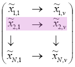
Just to summarize the way you do dimension reduction.  First you have X, and you remove the means.  On X you do a singular value decomposition and obtain matrices U, D, and V.  Then you call every column vector in V, \(v_j\), where j = 1, ... , p. This v_j is called the principal components direction.  Let's say your original dimension is 10 and we wish to reduce this to 2 dimensions, what would we do? We would take \(v_1\) and \(v_2\) and project X to \(v_1\) and X to \(v_2\).  To project, multiply X by \(v_1\) for a column vector of size N.  X times \(v_2\) gives you another column vector of size N.  These two column vectors reduce the dimensions so you have:

\[\begin{pmatrix}
\tilde{x}_{1,1} & \rightarrow & \tilde{x}_{1,v} \\
\tilde{x}_{2,1} & \rightarrow & \tilde{x}_{1,v} \\
\downarrow &  & \downarrow\\
\tilde{x}_{N,1} & \rightarrow & \tilde{x}_{N,v}
\end{pmatrix}\]

Every row would be a reduced version of your original data. If I asked you to give me the 2 dimensional version of the second sample point, then you would you would look at the row highlighted below: