GCD.1 - Exploratory Data Analysis (EDA) and Data Pre-processing
Before getting into any sophisticated analysis, the first step is to do an EDA and data cleaning. Since both categorical and continuous variables are included in the data set, appropriate tables and summary statistics are provided.
Sample R code for creating marginal proportional tables
Proportions of applicants belonging to each classification of a categorical variable are shown in the following table (below). The pink shadings indicate that these levels have too few observations and the levels are merged for final analysis.
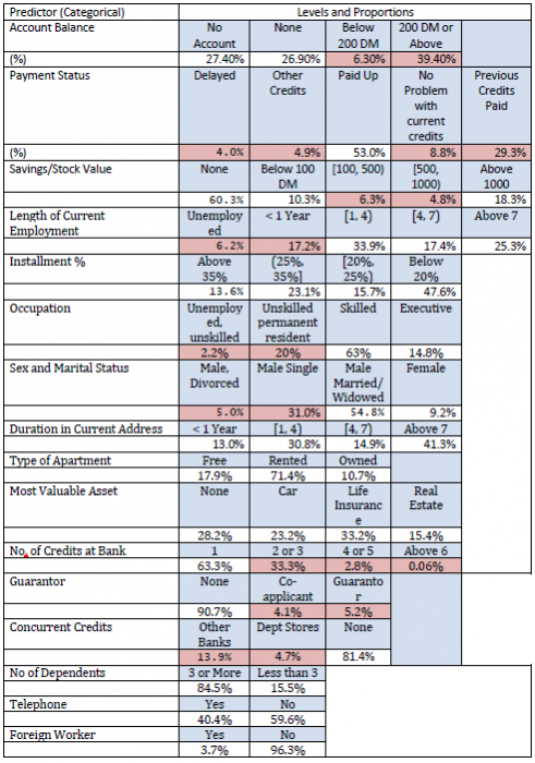
Since most of the predictors are categorical with several levels, the full cross-classification of all variables will lead to zero observations in many cells. Hence we need to reduce the table size. For details of variable names and classification see Appendix 1.
Depending on the cell proportions given in the one-way table above two or more cells are merged for several categorical predictors. We present below the final classification for the predictors that may potentially have any influence on Creditability
- Account Balance: No account (1), None (No balance) (2), Some Balance (3)
- Payment Status: Some Problems (1), Paid Up (2), No Problems (in this bank) (3)
- Savings/Stock Value: None, Below 100 DM, [100, 1000] DM, Above 1000 DM
- Employment Length: Below 1 year (including unemployed), [1, 4), [4, 7), Above 7
- Sex/Marital Status: Male Divorced/Single, Male Married/Widowed, Female
- No of Credits at this bank: 1, More than 1
- Guarantor: None, Yes
- Concurrent Credits: Other Banks or Dept Stores, None
- ForeignWorker variable may be dropped from the study
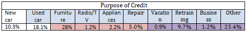
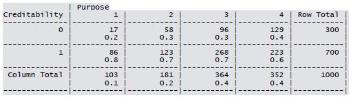
- Purpose of Credit: New car, Used car, Home Related, Other
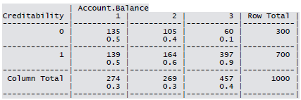
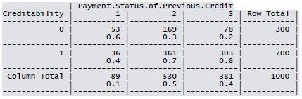
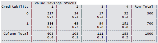
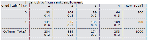
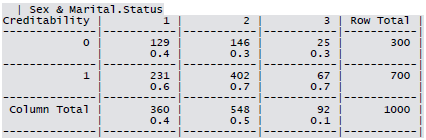
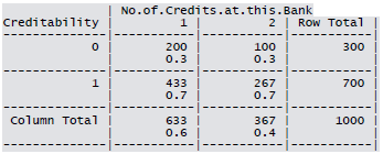
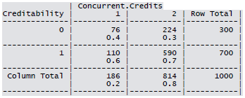
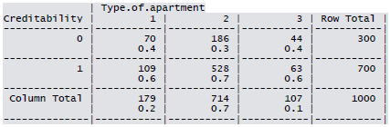
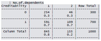
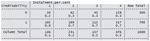
Cross-tabulation of the 9 predictors as defined above with Creditability is shown below. The proportions shown in the cells are column proportions and so are the marginal proportions. For example, 30% of 1000 applicants have no account and another 30% have no balance while 40% have some balance in their account. Among those who have no account 135 are found to be Creditable and 139 are found to be Non-Creditable. In the group with no balance in their account, 40% were found to be on-Creditable whereas in the group having some balance only 1% are found to be Non-Creditable.
Sample R code for creating K1 x K2 contingency table.

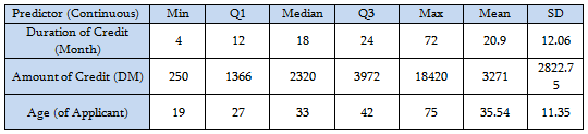
Summary for the continuous variables:
Sample R code for Descriptive Statistics.
Distribution of the continuous variables:
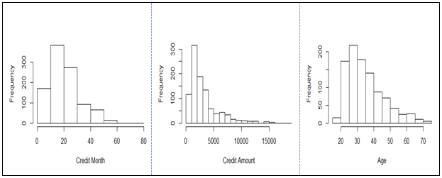
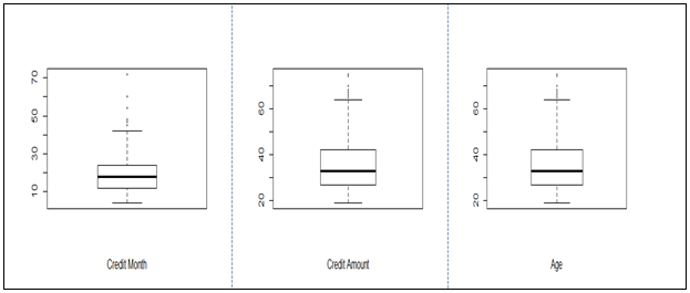
All the three variables show marked positive skewness. Boxplots bear this out even more clearly.
In preparation of predictors to use in building a logistic regression model, we consider bivariate association of the response (Creditability) with the categorical predictors.

