Printer-friendly version

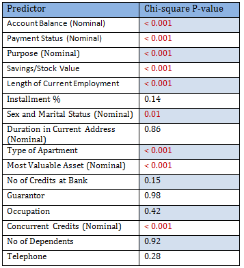
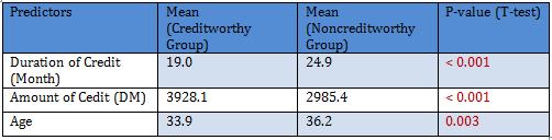
Since the number of predictors in this problem is not very high, it is possible to look into the dependency of the response (Creditability) on each of them individually. The following table summarizes the chi-square p-values for each contingency table. Note that among the sample of size 1000, 700 were Creditable and 300 Non-Creditable. This classification is based on the Bank’s opinion on the actual applicants.

Only significant predictors are to be included in the logistic regression model. Since there are 1000 observations 50:50 cross-validation scheme is tried:

Model Building with 50:50 Cross-validation

Sample R code for
50:50 cross-validation data creation.

indexes = sample(1:nrow(German.Credit), size=0.5*nrow(German.Credit)) # Random sample of 50% of row numbers created

Train50 <- German.Credit[indexes,] # Training data contains created indices

Test50 <- German.Credit[-indexes,] # Test data contains the rest

# Using any proportion, other than 0.5 above and size Training and Test data can be constructed

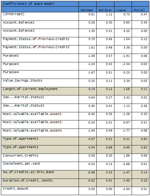
1000 observations are randomly partitioned into two equal sized subsets – Training and Test data. A logistic model is fit to the Training set.

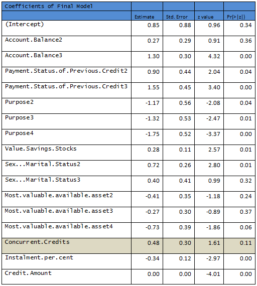
Results are given below, shaded rows indicate variables not significant at 10% level.

Sample R code for for
Logistic Model building with Training data
and assessing for Test data.

LogisticModel50 <- glm(Creditability ~ Account.Balance + Payment.Status.of.Previous.Credit + Purpose + Value.Savings.Stocks + Length.of.current.employment + Sex...Marital.Status + Most.valuable.available.asset + Type.of.apartment + Concurrent.Credits + Duration.of.Credit..month.+ Credit.Amount + Age..years., family=binomial, data = Train50)

LogisticModel50final <- glm(Creditability ~ Account.Balance + Payment.Status.of.Previous.Credit + Purpose + Length.of.current.employment + Sex...Marital.Status, family=binomial, data = Train50)

fit50 <- fitted.values(LogisticModel50S1)

Threshold50 <- rep(0,500)

for (i in 1:500)

if(fit50[i] >= 0.5) Threshold50[i] <- 1

CrossTable(Train50$Creditability, Threshold50, digits=1, prop.r=F, prop.t=F, prop.chisq=F, chisq=F, data=Train50)

perf <- performance(pred, "tpr", "fpr")

plot(perf)

R output:

Null deviance: 598.536 on 499 degrees of freedom
Residual deviance: 464.01 on 477 degrees of freedom
AIC: 510.01

 Removing the nonsignificant variables a second logistic regression is fit to the data.

R output:

Null deviance: 598.53 on 499 degrees of freedom
Residual deviance: 472.12 on 483 degrees of freedom
AIC: 506.12

Need to remove another variable to come up with a model where all predictors are significant at 10% level.

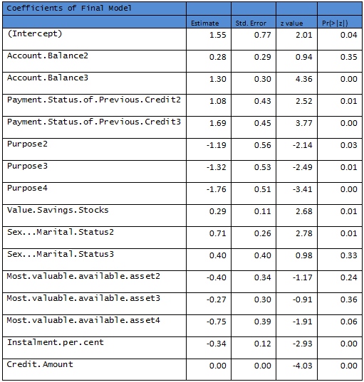
R output:

Null deviance: 598.53 on 499 degrees of freedom
Residual deviance: 474.67 on 484 degrees of freedom
AIC: 506.67

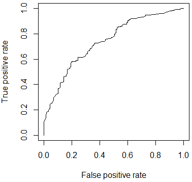
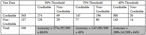
 This model is recommended as the final model based on the Training Data. Final performance of a model is evaluated by considering the classification power. Following are a few tables defined at different thresholds of classification.

Following figure shows the performance of the classifier through ROC curve.