10.5 - Uncorrelated Predictors
In order to get a handle on this multicollinearity thing, let's first investigate the effects that uncorrelated predictors have on regression analyses. To do so, we'll investigate a "contrived" data set, in which the predictors are perfectly uncorrelated. Then, we'll investigate a second example of a "real" data set, in which the predictors are nearly uncorrelated. Our two investigations will allow us to summarize the effects that uncorrelated predictors have on regression analyses.
Then, on the next page, we'll investigate the effects that highly correlated predictors have on regression analyses. In doing so, we'll learn — and therefore be able to summarize — the various effects multicollinearity has on regression analyses.
What is the effect on regression analyses if the predictors are perfectly uncorrelated?
Consider the following matrix plot of the response y and two predictors x1 and x2, of a contrived data set (uncorrpreds.txt), in which the predictors are perfectly uncorrelated:
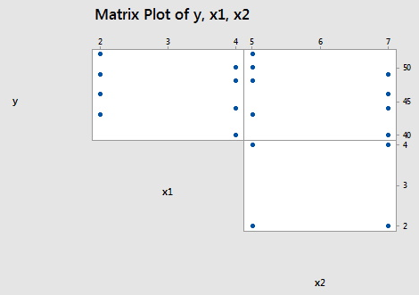
As you can see there is no apparent relationship at all between the predictors x1 and x2. That is, the correlation between x1 and x2 is zero:
![]()
suggesting the two predictors are perfectly uncorrelated.
Now, let's just proceed quickly through the output of a series of regression analyses collecting various pieces of information along the way. When we're done, we'll review what we learned by collating the various items in a summary table.
The regression of the response y on the predictor x1:
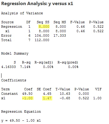
yields the estimated coefficient b1 = –1.00, the standard error se(b1) = 1.47, and the regression sum of squares SSR(x1) = 8.000.
The regression of the response y on the predictor x2:
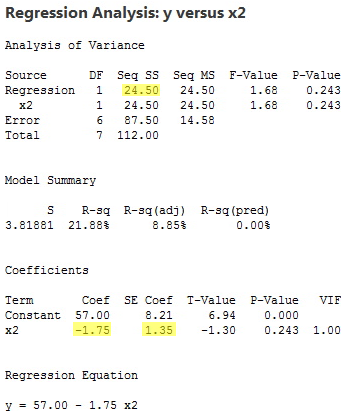
yields the estimated coefficient b2 = –1.75, the standard error se(b2) = 1.35, and the regression sum of squares SSR(x2) = 24.50.
The regression of the response y on the predictors x1 and x2 (in that order):
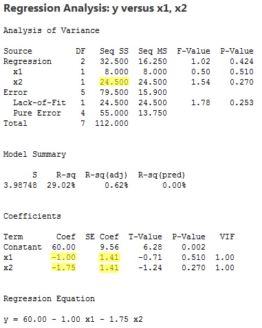
yields the estimated coefficients b1 = –1.00 and b2 = –1.75, the standard errors se(b1) = 1.41 and se(b2) = 1.41, and the sequential sum of squares SSR(x2|x1) = 24.500.
The regression of the response y on the predictors x2 and x1 (in that order):
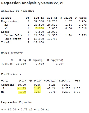
yields the estimated coefficients b1 = –1.00 and b2 = –1.75, the standard errors se(b1) = 1.41 and se(b2) = 1.41, and the sequential sum of squares SSR(x1|x2) = 8.000.
Okay — as promised — compiling the results in a summary table, we obtain:
|
Model |
b1
|
se(b1)
|
b2
|
se(b2)
|
Seq SS
|
|
x1 only
|
-1.00
|
1.47
|
---
|
---
|
SSR(x1)
8.000 |
|
x2 only
|
---
|
---
|
-1.75
|
1.35
|
SSR(x2)
24.50 |
|
x1, x2
(in order) |
-1.00
|
1.41
|
-1.75
|
1.41
|
SSR(x2|x1)
24.500 |
|
x2, x1
(in order) |
-1.00
|
1.41
|
-1.75
|
1.41
|
SSR(x1|x2)
8.000 |
What do we observe?
- The estimated slope coefficients b1 and b2 are the same regardless of the model used.
- The standard errors se(b1) and se(b2) don't change much at all from model to model.
- The sum of squares SSR(x1) is the same as the sequential sum of squares SSR(x1|x2). The sum of squares SSR(x2) is the same as the sequential sum of squares SSR(x2|x1).
These all seem to be good things! Because the slope estimates stay the same, the effect on the response ascribed to a predictor doesn't depend on the other predictors in the model. Because SSR(x1) = SSR(x1|x2), the marginal contribution that x1 has in reducing the variability in the response y doesn't depend on the predictor x2. Similarly, because SSR(x2) = SSR(x2|x1), the marginal contribution that x2 has in reducing the variability in the response y doesn't depend on the predictor x1.
These are the things we can hope for in a regression analyis —but, then reality sets in! Recall that we obtained the above results for a contrived data set, in which the predictors are perfectly uncorrelated. Do we get similar results for real data with only nearly uncorrelated predictors? Let's see!
What is the effect on regression analyses if the predictors are nearly uncorrelated?
To investigate this question, let's go back and take a look at the blood pressure data set (bloodpress.txt). In particular, let's focus on the relationships among the response y = BP and the predictors x3 = BSA and x6 = Stress:
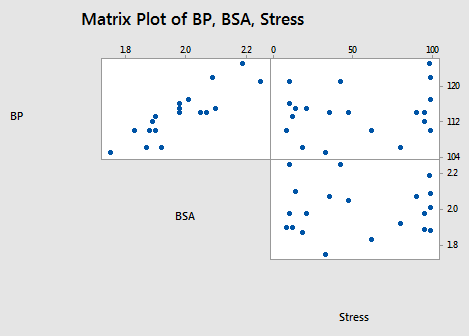
As the above matrix plot and the following correlation matrix suggest:
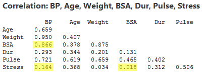
there appears to be a strong relationship between y = BP and the predictor x3 = BSA (r = 0.866), a weak relationship between y = BP and x6 = Stress (r = 0.164), and an almost non-existent relationship between x3 = BSA and x6 = Stress (r = 0.018). That is, the two predictors are nearly perfectly uncorrelated.
What effect do these nearly perfectly uncorrelated predictors have on regression analyses? Let's proceed similarly through the output of a series of regression analyses collecting various pieces of information along the way. When we're done, we'll review what we learned by collating the various items in a summary table.
The regression of the response y = BP on the predictor x6= Stress:
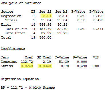
yields the estimated coefficient b6 = 0.0240, the standard error se(b6) = 0.0340, and the regression sum of squares SSR(x6) = 15.04.
The regression of the response y = BP on the predictor x3 = BSA:
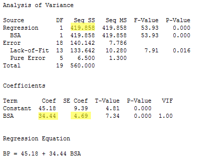
yields the estimated coefficient b3 = 34.44, the standard error se(b3) = 4.69, and the regression sum of squares SSR(x3) = 419.858.
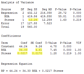
The regression of the response y = BP on the predictors x6= Stress and x3 = BSA (in that order):
yields the estimated coefficients b6 = 0.0217 and b3 = 34.33, the standard errors se(b6) = 0.0170 and se(b3) = 4.61, and the sequential sum of squares SSR(x3|x6) = 417.07.
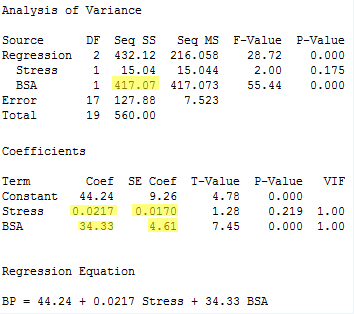
Finally, the regression of the response y = BP on the predictors x3 = BSA and x6= Stress (in that order):
yields the estimated coefficients b6 = 0.0217 and b3 = 34.33, the standard errors se(b6) = 0.0170 and se(b3) = 4.61, and the sequential sum of squares SSR(x6|x3) = 12.26.
Again — as promised — compiling the results in a summary table, we obtain:
|
Model |
b6
|
se(b6)
|
b3
|
se(b3)
|
Seq SS
|
|
x6 only
|
0.0240
|
0.0340
|
---
|
---
|
SSR(x6)
15.04 |
|
x3 only
|
---
|
---
|
34.44
|
4.69
|
SSR(x3)
419.858 |
|
x6, x3
(in order) |
0.0217
|
0.0170
|
34.33
|
4.61
|
SSR(x3|x6)
417.07 |
|
x3, x6
(in order) |
0.0217
|
0.0170
|
34.33
|
4.61
|
SSR(x6|x3)
12.26 |
What do we observe? If the predictors are nearly perfectly uncorrelated:
- We don't get identical, but very similar slope estimates b3 and b6, regardless of the predictors in the model.
- The sum of squares SSR(x3) is not the same, but very similar to the sequential sum of squares SSR(x3|x6).
- The sum of squares SSR(x6) is not the same, but very similar to the sequential sum of squares SSR(x6|x3).
Again, these are all good things! In short, the effect on the response ascribed to a predictor is similar regardless of the other predictors in the model. And, the marginal contribution of a predictor doesn't appear to depend much on the other predictors in the model.

