10.1 - Nonconstant Variance and Weighted Least Squares
Excessive nonconstant variance can create technical difficulties with a multiple linear regression model. For example, if the residual variance increases with the fitted values, then prediction intervals will tend to be wider than they should be at low fitted values and narrower than they should be at high fitted values. Some remedies for refining a model exhibiting excessive nonconstant variance includes the following:
- Apply a variance-stabilizing transformation to the response variable, for example a logarithmic transformation (or a square root transformation if a logarithmic transformation is "too strong" or a reciprocal transformation if a logarithmic transformation is "too weak"). We explored this in more detail in Lesson 7.
- Weight the variances so that they can be different for each set of predictor values. This leads to weighted least squares, in which the data observations are given different weights when estimating the model – see below.
- A generalization of weighted least squares is to allow the regression errors to be correlated with one another in addition to having different variances. This leads to generalized least squares, in which various forms of nonconstant variance can be modeled.
- For some applications we can explicitly model the variance as a function of the mean, E(Y). This approach uses the framework of generalized linear models, which we discuss in Lesson 12.
The method of ordinary least squares assumes that there is constant variance in the errors (which is called homoscedasticity). The method of weighted least squares can be used when the ordinary least squares assumption of constant variance in the errors is violated (which is called heteroscedasticity). The model under consideration is
\[\begin{equation*} \textbf{Y}=\textbf{X}\beta+\epsilon, \end{equation*}\]
where now \(\epsilon\) is assumed to be (multivariate) normally distributed with mean vector 0 and nonconstant variance-covariance matrix
\[\begin{equation*} \left(\begin{array}{cccc} \sigma^{2}_{1} & 0 & \ldots & 0 \\ 0 & \sigma^{2}_{2} & \ldots & 0 \\ \vdots & \vdots & \ddots & \vdots \\ 0 & 0 & \ldots & \sigma^{2}_{n} \\ \end{array} \right). \end{equation*}\]
If we define the reciprocal of each variance, \(\sigma^{2}_{i}\), as the weight, \(w_i = 1/\sigma^{2}_{i}\), then let matrix W be a diagonal matrix containing these weights:
\[\begin{equation*}\textbf{W}=\left( \begin{array}{cccc} w_{1} & 0 & \ldots & 0 \\ 0& w_{2} & \ldots & 0 \\ \vdots & \vdots & \ddots & \vdots \\ 0& 0 & \ldots & w_{n} \\ \end{array} \right). \end{equation*}\]
The weighted least squares estimate is then
\[\begin{align*} \hat{\beta}_{WLS}&=\arg\min_{\beta}\sum_{i=1}^{n}\epsilon_{i}^{*2}\\ &=(\textbf{X}^{T}\textbf{W}\textbf{X})^{-1}\textbf{X}^{T}\textbf{W}\textbf{Y}. \end{align*}\]
With this setting, we can make a few observations:
- Since each weight is inversely proportional to the error variance, it reflects the information in that observation. So, an observation with small error variance has a large weight since it contains relatively more information than an observation with large error variance (small weight).
- The weights have to be known (or more usually estimated) up to a proportionality constant.
To illustrate, consider the famous 1877 galton.txt dataset, consisting of 7 measurements each of X = Parent (pea diameter in inches of parent plant) and Y = Progeny (average pea diameter in inches of up to 10 plants grown from seeds of the parent plant). Also included in the dataset are standard deviations, SD, of the offspring peas grown from each parent. These standard deviations reflect the information in the response Y values (remember these are averages) and so in estimating a regression model we should downweight the obervations with a large standard deviation and upweight the observations with a small standard deviation. In other words we should use weighted least squares with weights equal to 1/SD2. The resulting fitted equation for this model is:
Progeny = 0.12796 + 0.2048 Parent
Compare this with the fitted equation for the ordinary least squares model:
Progeny = 0.12703 + 0.2100 Parent
The equations aren't very different but we can gain some intuition into the effects of using weighted least squares by looking at a scatterplot of the data with the two regression lines superimposed:
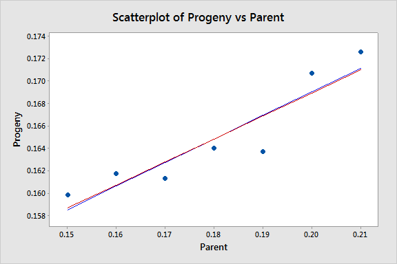
The blue line represents the OLS fit, while the red line represents the WLS fit. The standard deviations tend to increase as the value of Parent increases, so the weights tend to decrease as the value of Parent increases. Thus, on the left of the graph where the observations are upweighted the red fitted line is pulled slightly closer to the data points, whereas on the right of the graph where the observations are downweighted the red fitted line is slightly further from the data points.
For this example the weights were known. There are other circumstances where the weights are known:
- If the i-th response is an average of ni equally variable observations, then Var(yi) = \(\sigma^2/n_i\) and wi = ni.
- If the i-th response is a total of ni observations, then Var(yi) = \(n_i\sigma^2\) and wi =1/ ni.
- If variance is proportional to some predictor xi, then Var(yi) = \(x_i\sigma^2\) and wi =1/ xi.
In practice, for other types of dataset, the structure of W is usually unknown, so we have to perform an ordinary least squares (OLS) regression first. Provided the regression function is appropriate, the i-th squared residual from the OLS fit is an estimate of \(\sigma_i^2\) and the i-th absolute residual is an estimate of \(\sigma_i\) (which tends to be a more useful estimator in the presence of outliers). The residuals are much too variable to be used directly in estimating the weights, \(w_i,\) so instead we use either the squared residuals to estimate a variance function or the absolute residuals to estimate a standard deviation function. We then use this variance or standard deviation function to estimate the weights.
Some possible variance and standard deviation function estimates include:
- If a residual plot against a predictor exhibits a megaphone shape, then regress the absolute values of the residuals against that predictor. The resulting fitted values of this regression are estimates of \(\sigma_{i}\). (And remember \(w_i = 1/\sigma^{2}_{i}\)).
- If a residual plot against the fitted values exhibits a megaphone shape, then regress the absolute values of the residuals against the fitted values. The resulting fitted values of this regression are estimates of \(\sigma_{i}\).
- If a residual plot of the squared residuals against a predictor exhibits an upward trend, then regress the squared residuals against that predictor. The resulting fitted values of this regression are estimates of \(\sigma_{i}^2\).
- If a residual plot of the squared residuals against the fitted values exhibits an upward trend, then regress the squared residuals against the fitted values. The resulting fitted values of this regression are estimates of \(\sigma_{i}^2\).
After using one of these methods to estimate the weights, \(w_i\), we then use these weights in estimating a weighted least squares regression model. We consider some examples of this approach in the next section.
Some key points regarding weighted least squares are:
- The difficulty, in practice, is determining estimates of the error variances (or standard deviations).
- Weighted least squares estimates of the coefficients will usually be nearly the same as the "ordinary" unweighted estimates. In cases where they differ substantially, the procedure can be iterated until estimated coefficients stabilize (often in no more than one or two iterations); this is called iteratively reweighted least squares.
- In some cases, the values of the weights may be based on theory or prior research.
- In designed experiments with large numbers of replicates, weights can be estimated directly from sample variances of the response variable at each combination of predictor variables.
- Use of weights will (legitimately) impact the widths of statistical intervals.
 Example 1: Computer-Assisted Learning Dataset
The data below (ca_learning_new.txt) was collected from a study of computer-assisted learning by n = 12 students.
| i | Responses | Cost |
| 1 | 16 | 77 |
| 2 | 14 | 70 |
| 3 | 22 | 85 |
| 4 | 10 | 50 |
| 5 | 14 | 62 |
| 6 | 17 | 70 |
| 7 | 10 | 55 |
| 8 | 13 | 63 |
| 9 | 19 | 88 |
| 10 | 12 | 57 |
| 11 | 18 | 81 |
| 12 | 11 | 51 |
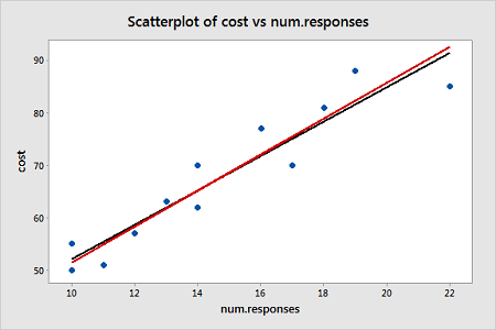
The response is the cost of the computer time (Y) and the predictor is the total number of responses in completing a lesson (X). A scatterplot of the data is given below.
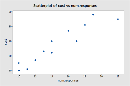
From this scatterplot, a simple linear regression seems appropriate for explaining this relationship.
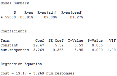
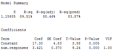
First an ordinary least squares line is fit to this data. Below is the summary of the simple linear regression fit for this data:
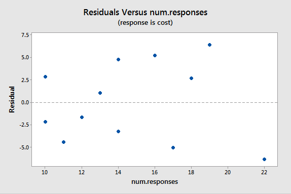
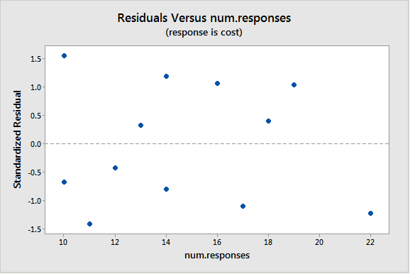
A plot of the residuals versus the predictor values indicates possible nonconstant variance since there is a very slight "megaphone" pattern:
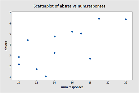
We will turn to weighted least squares to address this possiblity. The weights we will use will be based on regressing the absolute residuals versus the predictor. A plot of the absolute residuals versus the predictor values is as follows:
We therefore fit a simple linear regression model of the absolute residuals on the predictor and calculate weights as 1 over the squared fitted values from this model. Then we fit a weighted least squares regression model using the just-created weights. The summary of this weighted least squares fit is as follows:
Notice that the regression estimates have not changed much from the ordinary least squares method. The following plot shows both the OLS fitted line (black) and WLS fitted line (red) overlaid on the same scatterplot.
A plot of the standardized residuals versus the predictor values when using the weighted least squares method shows how we have corrected for the megaphone shape since the standardized residuals appear to be more randomly scattered about 0:
With weighted least squares, it is crucial that we use standardized residuals to evaluate the aptness of the model, since these take into account the weights that are used to model the changing variance. The usual residuals don't do this and will maintain the same non-constant variance pattern no matter which weights have been used in the analysis.
Example 2: Market Share Data
Here we have market share data for n = 36 consecutive months (marketshare.txt). Let Y = market share of the product; X1 = price; P1 = 1 if only a discount promotion is in effect and 0 otherwise; P2 = 1 if both discount and package promotions are in effect and 0 otherwise. The regression results below are for a useful model in this situation:
Analysis of Variance
Source      DF  Adj SS   Adj MS  F-Value  P-Value
Regression   3  1.7628  0.58761    27.51    0.000
Error       32  0.6834  0.02136
Total       35  2.4463

Model Summary
       S    R-sq  R-sq(adj)  R-sq(pred)
0.146141  72.06%     69.44%      64.70%

Coefficients
Term        Coef  SE Coef  T-Value  P-Value   VIF
Constant   3.196    0.356     8.97    0.000
Price     -0.334    0.152    -2.19    0.036  1.01
P1        0.3081   0.0641     4.80    0.000  1.20
P2        0.4843   0.0554     8.74    0.000  1.19
A residual plot suggests nonconstant variance related to whether or not a discount is in effect:
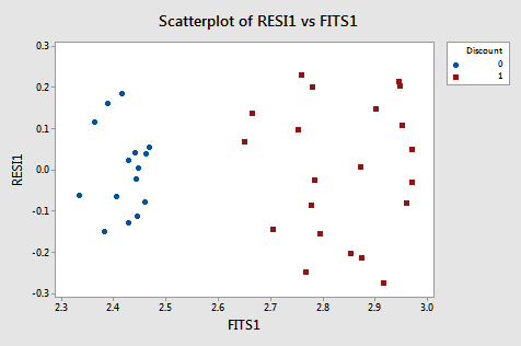
From this plot, it is apparent that the values coded as 0 have a smaller residual variance than the values coded as 1. The residual variances for the two separate groups defined by the discount pricing variable are:
Variable  Discount  Variance
RESI      0           0.0105
          1           0.0268
Because of this nonconstant variance, we will perform a weighted least squares analysis. For the weights, we use \(w_i=1 / \hat{\sigma}_i^2\) for i = 1, 2, i.e., 1/0.0105 for Discount=0 and 1/0.0268 for Discount=1, which could be expressed as "Discount/0.027 + (1–Discount)/0.0105." The weighted least squares analysis results using these weights is as follows:
Analysis of Variance
Source      DF   Adj SS  Adj MS  F-Value  P-Value
Regression   3   98.118  32.706    30.75    0.000
Error       32   34.031   1.063
Total       35  132.149

Model Summary
      S    R-sq  R-sq(adj)  R-sq(pred)
1.03125  74.25%     71.83%      67.96%

Coefficients
Term        Coef  SE Coef  T-Value  P-Value   VIF
Constant   3.174    0.357     8.90    0.000
Price     -0.324    0.153    -2.12    0.042  1.01
P1        0.3083   0.0658     4.69    0.000  1.05
P2        0.4842   0.0542     8.93    0.000  1.05
An important note is that the ANOVA table will be in terms of the weighted SS. When doing a weighted least squares analysis, you should note how different the SS values of the weighted case are from the SS values for the unweighted case.
Also, note again how the regression coefficients of the weighted case are not much different from those in the unweighted case. Thus, there may not appear to be much of an obvious benefit to using the weighted analysis, but keep in mind that prediction intervals are going to be more reflective of the data.
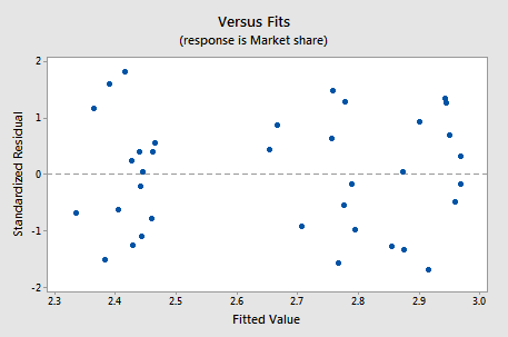
If you proceed with a weighted least squares analysis, you should check a plot of the residuals again. Remember to use the standardized residuals when doing so! For this example, the plot of standardized residuals after doing a weighted least squares analysis is given below and the residuals look okay.
 Example 3: Home Price Dataset
This dataset (realestate.txt) has the following variables:
Y = sale price of home
X1 = square footage of home
X2 = square footage of the lot
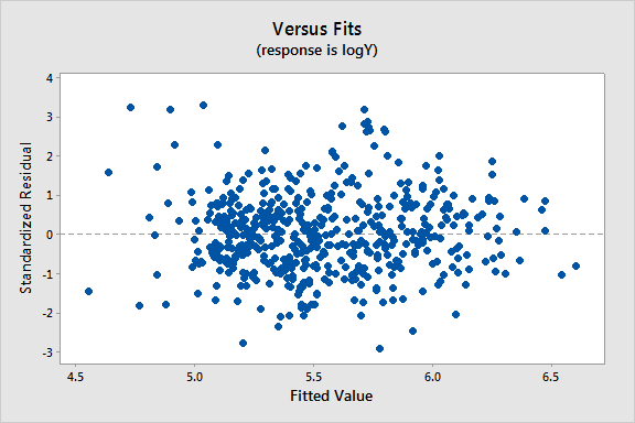
Since all the variables are highly skewed we first transform each variable to its natural logarithm. Then when we perform a regression analysis and look at a plot of the residuals versus the fitted values (see below), we note a slight “megaphone” or “conic” shape of the residuals.
Term        Coef  SE Coef  T-Value  P-Value   VIF
Constant  4.2548   0.0735    57.86    0.000
logX1     1.2214   0.0337    36.23    0.000  1.05
logX2     0.1059   0.0239     4.42    0.000  1.05
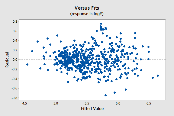
We interpret this plot as having a mild pattern of nonconstant variance in which the amount of variation is related to the size of the mean, E(Y) (which is estimated by the fits).
So, we use the following procedure to determine appropriate weights:
- Store the residuals and the fitted values from the ordinary least squares (OLS) regression.
- Calculate the absolute values of the OLS residuals.
- Regress the absolute values of the OLS residuals versus the OLS fitted values and store the fitted values from this regression. These fitted values are estimates of the error standard deviations.
- Calculate weights equal to 1/fits2, where "fits" are the fitted values from the regression in the last step.
We then refit the original regression model but using these weights in a weighted least squares (WLS) regression.
Results and a residual plot for this WLS model indicate the nonconstant variance problem has been mitigated to some extent:
Term        Coef  SE Coef  T-Value  P-Value   VIF
Constant  4.3519   0.0633    68.75    0.000
logX1     1.2015   0.0333    36.06    0.000  1.08
logX2     0.0792   0.0215     3.68    0.000  1.08