Next, let us consider the problem in which we have a y-variable and x-variables all measured as a time series. As an example, we might have y as the monthly highway accidents on an interstate highway and x as the monthly amount of travel on the interstate, with measurements observed for 120 consecutive months. A multiple (time series) regression model can be written as:

\[\begin{equation} y_{t}=\textbf{X}_{t}\beta+\epsilon_{t}. \end{equation}\]

The difficulty that often arises in this context is that the errors (\(\epsilon_{t}\)) may be correlated with each other. In other words, we have autocorrelation or dependency between the errors.

We may consider situations in which the error at one specific time is linearly related to the error at the previous time. That is, the errors themselves follow a simple linear regression model that can be written as

\[\begin{equation} \epsilon_{t}=\rho\epsilon_{t-1}+\omega_{t}. \end{equation}\]

Here, \(|\rho|<1 \) is called the autocorrelation parameter and the \(\omega_{t}\) term is a new error term that follows the usual assumptions that we make about regression errors: \(\omega_{t}\sim_{iid}N(0,\sigma^{2})\). (Here "iid" stands for "independent and identically distributed.) So, this model says that the error at time t is a fraction of the error at time t - 1 plus some new perturbation \(\omega_{t}\).

Our model for the \(\epsilon_{t}\) errors of the original Y versus X regression is an autoregressive model for the errors, specifically AR(1) in this case. One reason why the errors might have an autoregressive structure is that the Y and X variables at time t may be (and most likely are) related to the Y and X measurements at time t – 1. These relationships are being absorbed into the error term of our multiple linear regression model that only relates Y and X measurements made at concurrent times. Notice that the autoregressive model for the errors is a violation of the assumption that we have independent errors and this creates theoretical difficulties for ordinary least squares estimates of the beta coefficients. There are several different methods for estimating the regression parameters of the Y versus X relationship when we have errors with an autoregressive structure and we will introduce a few of these methods later.

The error terms \(\epsilon_{t}\) still have mean 0 and constant variance:

\[\begin{align*} \mbox{E}(\epsilon_{t})&=0 \\ \mbox{Var}(\epsilon_{t})&=\frac{\sigma^{2}}{1-\rho^{2}}. \end{align*}\]

However, the covariance between adjacent error terms is:

\[\begin{equation*} \mbox{Cov}(\epsilon_{t},\epsilon_{t-1})=\rho\biggl(\frac{\sigma^{2}}{1-\rho^{2}}\biggr), \end{equation*}\]

which implies the correlation between adjacent error terms is:

\[\begin{equation*} \mbox{Corr}(\epsilon_{t},\epsilon_{t-1})=\frac{\mbox{Cov}(\epsilon_{t},\epsilon_{t-1})}{\sqrt{\mbox{Var}(\epsilon_{t})\mbox{Var}(\epsilon_{t-1})}}=\rho, \end{equation*}\]

which is the autocorrelation parameter we introduced above.

We can use partial autocorrelation function (PACF) plots to help us assess appropriate lags for the errors in a regression model with autoregressive errors. Specifically, we first fit a multiple linear regression model to our time series data and store the residuals. Then we can look at a plot of the PACF for the residuals versus the lag. Large sample partial autocorrelations that are significantly different from 0 indicate lagged terms of \(\epsilon\) that may be useful predictors of \(\epsilon_{t}\).

Here we present some formal tests and remedial measures for dealing with error autocorrelation.

Durbin-Watson Test

If we suspect first-order autocorrelation with the errors, then one formal test regarding the parameter \(\rho\) is the Durbin-Watson test:

\[\begin{align*} \nonumber H_{0}&: \rho=0 \\ \nonumber H_{A}&: \rho\neq 0. \end{align*}\]

The null hypothesis of \(\rho=0\) implies that \(\epsilon_{t}=\omega_{t}\), or that the error term in one period is not correlated with the error term in the previous period. The alternative hypothesis of \(\rho\neq 0\) means the error term in one period is either positively or negatively correlated with the error term in the previous period. Often times, a researcher will already have an indication of whether the errors are positively or negatively correlated. For example, a regression of oil prices (in dollars per barrel) versus the gas price index will surely have positively correlated errors. When the researcher has an indication of the direction of the correlation, then the Durbin-Watson test also accommodates the one-sided alternatives \(H_{A}:\rho< 0\) for negative correlations or \(H_{A}:\rho> 0\) for positive correlations (as in the oil example).

The test statistic for the Durbin-Watson test on a data set of size n is given by:

\[\begin{equation*} D=\frac{\sum_{t=2}^{n}(e_{t}-e_{t-1})^{2}}{\sum_{t=1}^{n}e_{t}^{2}}, \end{equation*}\]

where \(e_{t}=y_{t}-\hat{y}_{t}\) are the residuals from the ordinary least squares fit. Exact critical values are difficult to obtain, but tables (for certain significance values) can be used to make a decision (e.g., see the tables at this link). The tables provide a lower and upper bound, called \(d_{L}\) and \(d_{U}\), respectively. In testing for positive autocorrelation, if \(D<d_{L}\) then reject \(H_{0}\), if \(D>d_{U}\) then fail to reject \(H_{0}\), or if \(d_{L}\leq D\leq d_{U}\), then the test is inconclusive. While the prospect of having an inconclusive test result is less than desirable, there are some programs which use exact and approximate procedures for calculating a p-value. These procedures require certain assumptions on the data which we will not discuss.

To illustrate, consider the Blaisdell Company example from page 489 of Applied Linear Regression Models (4th ed) by Kutner, Nachtsheim, and Neter. If we fit a simple linear regression model with response comsales (company sales in $ millions) and predictor indsales (industry sales in $ millions) we obtain the following output for the Durbin-Watson test:

Term         Coef  SE Coef  T-Value  P-Value   VIF
Constant   -1.455    0.214    -6.79    0.000
indsales  0.17628  0.00144   122.02    0.000  1.00

Durbin-Watson Statistic =  0.734726

Since the value of the Durbin-Watson Statistic falls below the lower bound at a 0.01 significance level (obtained from a table of Durbin-Watson test bounds), there is strong evidence the error terms are positively correlated.

Ljung-Box Q Test

The Ljung-Box Q test (sometimes called the Portmanteau test) is used to test whether or not observations over time are random and independent. In particular, for a given k, it tests the following:

\[\begin{align*} \nonumber H_{0}&: \textrm{the autocorrelations up to lag} \ k \ \textrm{are all 0} \\ \nonumber H_{A}&: \textrm{the autocorrelations of one or more lags differ from 0}. \end{align*}\]

The test statistic is calculated as:

\[\begin{equation*} Q_{k}=n(n+2)\sum_{j=1}^{k}\frac{{r}^{2}_{j}}{n-j}, \end{equation*}\]

which is approximately \(\chi^{2}_{k}\)-distributed.

To illustrate how the test works for k=1, consider the Blaisdell Company example from above. If we store the residuals from a simple linear regression model with response comsales and predictor indsales, we obtain the following output for the autocorrelation function for the residuals and the Ljung-Box Q test:

Autocorrelation Function: RESI1
Lag        ACF      T    LBQ
  1   0.626005   2.80   9.08

The Ljung-Box Q test statistic of 9.08 corresponds to a \(\chi^{2}_{1}\) p-value of 0.0026, so there is strong evidence the lag-1 autocorrelation is non-zero.

Remedial Measures

When autocorrelated error terms are found to be present, then one of the first remedial measures should be to investigate the omission of a key predictor variable. If such a predictor does not aid in reducing/eliminating autocorrelation of the error terms, then certain transformations on the variables can be performed. We discuss three transformations that are designed for AR(1) errors. Methods for dealing with errors from an AR(k) process do exist in the literature, but are much more technical in nature.

Cochrane-Orcutt Procedure

The first of the three transformation methods we discuss is called the Cochrane-Orcutt procedure, which involves an iterative process (after identifying the need for an AR(1) process):

Estimate \(\rho\) for \[\begin{equation*} \epsilon_{t}=\rho\epsilon_{t-1}+\omega_{t} \end{equation*}\] by performing a regression through the origin. Call this estimate r.

Transform the variables from the multiple regression model \[\begin{equation*} y_{t}=\beta_{0}+\beta_{1}x_{t,1}+\ldots+\beta_{k}x_{t,k}+\epsilon_{t} \end{equation*}\] by setting \(y_{t}^{*}=y_{t}-ry_{t-1}\) and \(x_{t,j}^{*}=x_{t,j}-rx_{t-1,j}\) for \(j=1,\ldots,k\).

Regress \(y_{t}^{*}\) on the transformed predictors using ordinary least squares to obtain estimates \(\hat{\beta}_{0}^{*},\ldots,\hat{\beta}_{k}^{*}\). Look at the error terms for this fit and determine if autocorrelation is still present (e.g., using the Durbin-Watson test). If autocorrelation is still present, then iterate this procedure. When the autocorrelation appears to be corrected, then transform the estimates back to their original scale by setting \(\hat{\beta}_{0}=\hat{\beta}_{0}^{*}/(1-r)\) and \(\hat{\beta}_{j}=\hat{\beta}_{j}^{*}\) for \(j=1,\ldots,k\). Notice that only the intercept parameter requires a transformation. Furthermore, the standard errors of the regression estimates for the original scale can also be obtained by setting \(\textrm{s.e.}(\hat{\beta}_{0})=\textrm{s.e.}(\hat{\beta}_{0}^{*})/(1-r)\) and \(\textrm{s.e.}(\hat{\beta}_{j})=\textrm{s.e.}(\hat{\beta}_{j}^{*})\) for \(j=1,\ldots,k\).

To illustrate the Cochrane-Orcutt prcedure, consider the Blaisdell Company example from above:

• Store the residuals, RESI, from a simple linear regression model with response comsales and predictor indsales.
• Calculate a lag-1 residual variable, lagRESI.
• Fit a simple linear regression model with response RESI and predictor lagRESI and no intercept. The estimated slope from this regression, 0.631164, is an estimate of the autocorrelation parameter, \(\rho\).
• Calculate a transformed response variable, Y_co = comsales-0.631164*LAG(comsales,1).
• Calculate a transformed predictor variable, X_co = indsales-0.631164*LAG(indsales,1).
• Fit a simple linear regression model with response Y_co and predictor X_co to obtain the following output:

Term         Coef  SE Coef  T-Value  P-Value   VIF
Constant   -0.394    0.167    -2.36    0.031
X_co      0.17376  0.00296    58.77    0.000  1.00

Durbin-Watson Statistic =  1.65025

• Since the value of the Durbin-Watson Statistic falls above the upper bound at a 0.01 significance level (obtained from a table of Durbin-Watson test bounds), there is no evidence the error terms are positively correlated in the model with the transformed variables.
• Transform the intercept parameter, -0.394/(1-0.631164) = -1.068, and its standard error, 0.167/(1-0.631164) = 0.453 (the slope estimate and standard error don't require transforming).
• The fitted regression function for the original variables is predicted comsales = -1.068 + 0.17376 indsales.
  

One thing to note about the Cochrane-Orcutt approach is that it does not always work properly. This occurs primarily because if the errors are positively autocorrelated, then r tends to underestimate \(\rho\). When this bias is serious, then it can seriously reduce the effectiveness of the Cochrane-Orcutt procedure.

Hildreth-Lu Procedure

The Hildreth-Lu procedure is a more direct method for estimating \(\rho\). After establishing that the errors have an AR(1) structure, follow these steps:

1. Select a series of candidate values for \(\rho\) (presumably values that would make sense after you assessed the pattern of the errors).
2. For each candidate value, regress \(y_{t}^{*}\) on the transformed predictors using the transformations established in the Cochrane-Orcutt procedure. Retain the SSEs for each of these regressions.
3. Select the value which minimizes the SSE as an estimate of \(\rho\).

Notice that this procedure is similar to the Box-Cox transformation discussed previously and that it is not iterative like the Cochrane-Orcutt procedure.

To illustrate the Hildreth-Lu procedure, consider the Blaisdell Company example from above:

• Calculate a transformed response variable, Y_hl.1 = comsales-0.1*LAG(comsales,1).
• Calculate a transformed predictor variable, X_hl.1 = indsales-0.1*LAG(indsales,1).
• Fit a simple linear regression model with response Y_hl.1 and predictor X_hl.1 and record the SSE.
• Repeat steps 1-3 for a series of estimates of \(\rho\) to find when SSE is minimized (0.96 leads to the minimum in this case).
• The output for this model is:

Analysis of Variance
Source      DF   Adj SS   Adj MS  F-Value  P-Value
Regression   1  2.31988  2.31988   550.26    0.000
  X_hl.96    1  2.31988  2.31988   550.26    0.000
Error       17  0.07167  0.00422
Total       18  2.39155
 
Term         Coef  SE Coef  T-Value  P-Value   VIF
Constant   0.0712   0.0580     1.23    0.236
X_hl.96   0.16045  0.00684    23.46    0.000  1.00

Durbin-Watson Statistic =  1.72544

• Since the value of the Durbin-Watson Statistic falls above the upper bound at a 0.01 significance level (obtained from a table of Durbin-Watson test bounds), there is no evidence the error terms are positively correlated in the model with the transformed variables.
• Transform the intercept parameter, 0.0712/(1-0.96) = 1.78, and its standard error, 0.0580/(1-0.96) = 1.45 (the slope estimate and standard error don't require transforming).
• The fitted regression function for the original variables is predicted comsales = 1.78 + 0.16045 indsales.
  

First Differences Procedure

Since \(\rho\) is frequently large for AR(1) errors (especially in economics data), many have suggested just setting \(\rho\) = 1 in the transformed model of the previous two procedures. This procedure is called the first differences procedure and simply regresses \(y_{t}^{*}=y_{t}-y_{t-1}\) on the \(x_{t,j}^{*}=x_{t,j}-x_{t-1,j}\) for \(j=1,\ldots,k\). The estimates from this regression are then transformed back, setting \(\hat{\beta}_{j}=\hat{\beta}_{j}^{*}\) for \(j=1,\ldots,k\) and \(\hat{\beta}_{0}=\bar{y}-(\hat{\beta}_{1}\bar{x}_{1}+\ldots+\hat{\beta}_{k}\bar{x}_{k})\).

To illustrate the first differences procedure, consider the Blaisdell Company example from above:

• Calculate a transformed response variable, Y_fd = comsales-LAG(comsales,1).
• Calculate a transformed predictor variable, X_fd = indsales-LAG(indsales,1).
• Fit a simple linear regression model with response Y_fd and predictor X_fd and find the Durbin-Watson statistic:

Durbin-Watson Statistic =  1.74883

• Since the value of the Durbin-Watson Statistic falls above the upper bound at a 0.01 significance level (obtained from a table of Durbin-Watson test bounds), there is no evidence the error terms are correlated in the model with the transformed variables.
• Fit a simple linear regression model with response Y_fd and predictor X_fd and no intercept. The output for this model is:

Term     Coef  SE Coef  T-Value  P-Value   VIF
X_fd  0.16849  0.00510    33.06    0.000  1.00

• Find the sample mean of comsales and indsales:

Variable   N  N*    Mean  SE Mean  StDev  Minimum      Q1  Median      Q3  Maximum
comsales  20   0  24.569    0.539  2.410   20.960  22.483  24.200  26.825   28.780
indsales  20   0  147.62     3.06  13.67   127.30  135.53  145.95  159.85   171.70

• Calculate the intercept parameter, 24.569 - 0.16849(147.62) = -0.303.
• The fitted regression function for the original variables is predicted comsales = -0.303 + 0.16849 indsales.

Forecasting Issues

When calculating forecasts for regression with autoregressive errors, it is important to utilize the modeled error structure as part of our process. For example, for AR(1) errors, \(\epsilon_{t}=\rho\epsilon_{t-1}+\omega_{t}\), our fitted regression equation is

\[\begin{equation*} \hat{y}_{t}=b_{0}+b_{1}x_{t}, \end{equation*}\]

with forecasts of \(y\) at time \(t\), denoted \(F_{t}\), computed as:

\[\begin{equation*} F_{t}=\hat{y}_{t}+e_{t}=\hat{y}_{t}+re_{t-1}. \end{equation*}\]

So, we can compute forecasts of \(y\) at time \(t+1\), denoted \(F_{t+1}\), iteratively:

• Compute the fitted value for time period t, \(\hat{y}_{t}=b_{0}+b_{1}x_{t}\)
• Compute the residual for time period t, \(e_{t}=y_{t}-\hat{y}_{t}\).
• Compute the fitted value for time period t+1, \(\hat{y}_{t+1}=b_{0}+b_{1}x_{t+1}\).
• Compute the forecast for time period t+1, \(F_{t+1}=\hat{y}_{t+1}+re_{t}\).
• Iterate.

To illustrate forecasting for the Cochrane-Orcutt procedure, consider the Blaisdell Company example from above. Suppose we wish to forecast comsales for time period 21 when indsales are projected to be $175.3 million:

• The fitted value for time period 20 is \(\hat{y}_{20} = -1.068+0.17376(171.7)) = 28.767\).
• The residual for time period 20 is \(e_{20} = y_{20}-\hat{y}_{20} = 28.78 - 28.767 = 0.013\).
• The fitted value for time period 21, \(\hat{y}_{21} = -1.068+0.17376(175.3)) = 29.392\).
• The forecast for time period 21 is \(F_{21}=29.392+0.631164(0.013)=29.40\).

Note that this procedure is not needed when simply using the lagged response variable as a predictor, e.g., in the first order autoregression model

\[\begin{equation*} y_{t}=\beta_{0}+\beta_{1}y_{t-1}+\epsilon_{t} \end{equation*}.\]

Example: Employee Data

The next data set gives the number of employees (in thousands) for a metal fabricator and one of their primary vendors for each month over a 5-year period, so n = 60 (employee.txt). A simple linear regression analysis was implemented:

\[\begin{equation*} y_{t}=\beta_{0}+\beta_{1}x_{t}+\epsilon_{t}, \end{equation*}\]

where \(y_{t}\) and \(x_{t}\) are the number of employees during time period t at the metal fabricator and vendor, respectively.

A plot of the number of employees at the fabricator versus the number of employees at the vendor with the ordinary least squares regression line overlaid is given below in plot (a). A scatterplot of the residuals versus t (the time ordering) is given in plot (b).

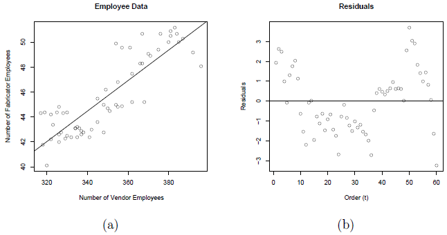
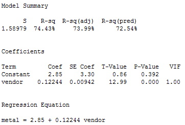
Notice the non-random trend suggestive of autocorrelated errors in the residual plot. The estimated equation is \(y_{t}=2.85+0.12244x_{t}+e_{t}\), which is given in the following summary output:

The plot below gives the PACF plot of the residuals, which helps us decide the lag values.

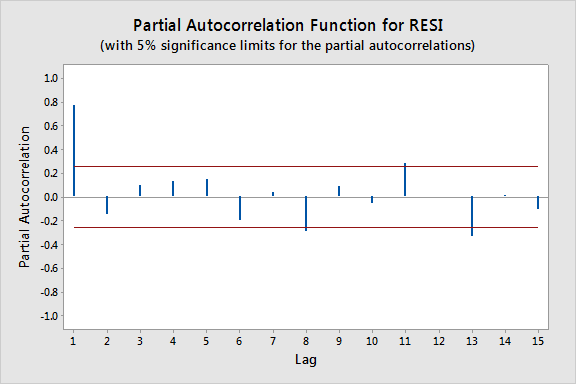
(a) Autocorrelations and (b) partial autocorrelations versus lag for the residuals from the employee data set.

In particular, it looks there is a lag of 1 since the lag-1 partial autocorrelation is so large and way beyond the "5% significance limits" shown by the red lines. (The partial autocorrelations at lags 8, 11, and 13 are only slightly beyond the limits and would lead to an overly complex model at this stage of the analysis.) We can also obtain the output from the Durbin-Watson test for serial correlation: 

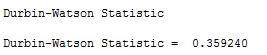
To find the p-value for this test statistic we need to look up a Durbin-Watson critical values table, which in this case indicates a highly significant p-value of approximately 0. (In general Durbin-Watson statistics close to 0 suggest significant positive autocorrelation.) A lag of 1 appears appropriate.

Since we decide upon using AR(1) errors, we will have to use one of the procedures we discussed earlier. In particular, we will use the Cochrane-Orcutt procedure.  Start by fitting a simple linear regression model with response variable equal to the residuals from the model above and predictor variable equal to the lag-1 residuals and no intercept to obtain the slope estimate, r = 0.831385.

Now, transform to \(y_{t}^{*}=y_{t}-ry_{t-1}\) and \(x_{t}^{*}=x_{t}-rx_{t-1}\). Perform a simple linear regression of \(y_{t}^{*}\) on \(x_{t}^{*}\). The resulting regression estimates from the Cochrane-Orcutt procedure are:

\[\begin{align*} \hat{\beta}_{1}^{*}&=0.0479=\hat{\beta}_{1} \\ \hat{\beta}_{0}^{*}&=4.876\Rightarrow\hat{\beta}_{0}=\frac{4.876}{1-0.831385}=28.918. \end{align*}\]

The corresponding standard errors are:

\[\begin{align*} \mbox{s.e.}(\hat{\beta}_{1}^{*})&=0.0130=\mbox{s.e.}(\hat{\beta}_{1})\\ \mbox{s.e.}(\hat{\beta}_{0}^{*})&=0.787\Rightarrow\mbox{s.e.}(\hat{\beta}_{0})=\frac{0.787}{1-0.831385}=4.667. \end{align*}\]

Notice that the correct standard errors (from the Cochrane-Orcutt procedure) are larger than the incorrect values from the simple linear regression on the original data. If ordinary least squares estimation is used when the errors are autocorrelated, the standard errors often are underestimated. It is also important to note that this does not always happen. Overestimation of the standard errors is an "on average" tendency over all problems.