One common way for the "independence" condition in a multiple linear regression model to fail is when the sample data have been collected over time and the regression model fails to effectively capture any time trends. In such a circumstance, the random errors in the model are often positively correlated over time, so that each random error is more likely to be similar to the previous random error that it would be if the random errors were independent of one another. This phenomenon is known as autocorrelation (or serial correlation) and can sometimes be detected by plotting the model residuals versus time. We'll explore this further in this section and the next.

A time series is a sequence of measurements of the same variable(s) made over time. Usually the measurements are made at evenly spaced times - for example, monthly or yearly. Let us first consider the problem in which we have a y-variable measured as a time series. As an example, we might have y a measure of global temperature, with measurements observed each year. To emphasize that we have measured values over time, we use "t" as a subscript rather than the usual "i," i.e., \(y_t\) means \(y\) measured in time period \(t\). An autoregressive model is when a value from a time series is regressed on previous values from that same time series. for example, \(y_{t}\) on \(y_{t-1}\):

\[\begin{equation*} y_{t}=\beta_{0}+\beta_{1}y_{t-1}+\epsilon_{t}. \end{equation*}\]

In this regression model, the response variable in the previous time period has become the predictor and the errors have our usual assumptions about errors in a simple linear regression model. The order of an autoregression is the number of immediately preceding values in the series that are used to predict the value at the present time. So, the preceding model is a first-order autoregression, written as AR(1).

If we want to predict \(y\) this year (\(y_{t}\)) using measurements of global temperature in the previous two years (\(y_{t-1},y_{t-2}\)), then the autoregressive model for doing so would be:

\[\begin{equation*} y_{t}=\beta_{0}+\beta_{1}y_{t-1}+\beta_{2}y_{t-2}+\epsilon_{t}. \end{equation*}\]

This model is a second-order autoregression, written as AR(2), since the value at time $t$ is predicted from the values at times \(t-1\) and \(t-2\). More generally, a \(k^{\textrm{th}}\)-order autoregression, written as AR(k), is a multiple linear regression in which the value of the series at any time t is a (linear) function of the values at times \(t-1,t-2,\ldots,t-k\).

Autocorrelation and Partial Autocorrelation

The coefficient of correlation between two values in a time series is called the autocorrelation function (ACF) For example the ACF for a time series \(y_t\) is given by:

\[\begin{equation*} \mbox{Corr}(y_{t},y_{t-k}), k=1, 2, .... \end{equation*}\]

This value of k is the time gap being considered and is called the lag. A lag 1 autocorrelation (i.e., k = 1 in the above) is the correlation between values that are one time period apart. More generally, a lag k autocorrelation is the correlation between values that are k time periods apart.

The ACF is a way to measure the linear relationship between an observation at time t and the observations at previous times. If we assume an AR(k) model, then we may wish to only measure the association between \(y_{t}\) and \(y_{t-k}\) and filter out the linear influence of the random variables that lie in between (i.e., \(y_{t-1},y_{t-2},\ldots,y_{t-(k-1 )}\)), which requires a transformation on the time series. Then by calculating the correlation of the transformed time series we obtain the partial autocorrelation function (PACF).

The PACF is most useful for identifying the order of an autoregressive model. Specifically, sample partial autocorrelations that are significantly different from 0 indicate lagged terms of \(y\) that are useful predictors of \(y_{t}\). It is important that the choice of the order makes sense. For example, suppose you have blood pressure readings for every day over the past two years. You may find that an AR(1) or AR(2) model is appropriate for modeling blood pressure. However, the PACF may indicate a large partial autocorrelation value at a lag of 17, but such a large order for an autoregressive model likely does not make much sense.

Example 1: Google Data

The data set (google_stock.txt) consists of n = 105 values which are the closing stock price of a share of Google stock during 2-7-2005 to 7-7-2005. We will analyze the dataset to identify the order of an autoregressive model. A plot of the stock prices versus time is presented in the figure below:

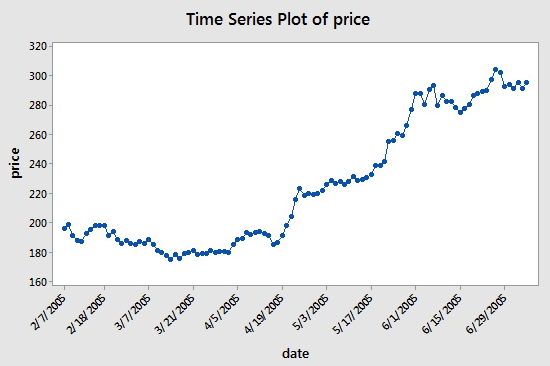
Consecutive values appear to follow one another fairly closely, suggesting an autoregression model could be appropriate. We next look at a plot of partial autocorrelations for the data:

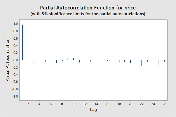
Here we notice that there is a significant spike at a lag of 1 and much lower spikes for the subsequent lags. Thus, an AR(1) model would likely be feasible for this data set.

Approximate bounds can also be constructed (as given by the red lines in the plot above) for this plot to aid in determining large values. Approximate \((1-\alpha)\times 100\%\) significance bounds are given by \(\pm z_{1-\alpha/2}/\sqrt{n}\). Values lying outside of either of these bounds are indicative of an autoregressive process.

We next create a lag-1 price variable and consider a scatterplot of price versus this lag-1 variable:

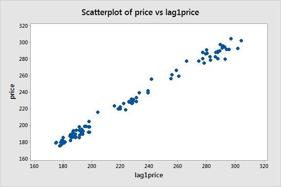
There appears to be a strong linear pattern, affirming that the first-order autoregression model

\[\begin{equation*} y_{t}=\beta_{0}+\beta_{1}y_{t-1}+\epsilon_{t} \end{equation*}\]

could be useful.

Example 2: Quake Data

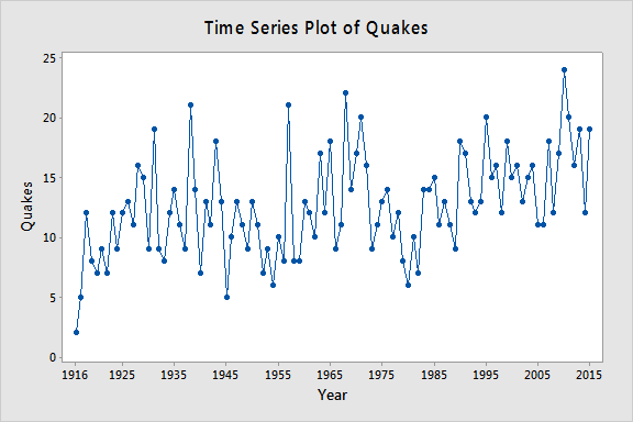
Let y_t = the annual number of worldwide earthquakes with magnitude greater than 7 on the Richter scale for n = 100 years (earthquakes.txt data obtained from https://earthquake.usgs.gov). The plot below gives a time series plot for this dataset.

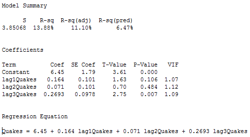
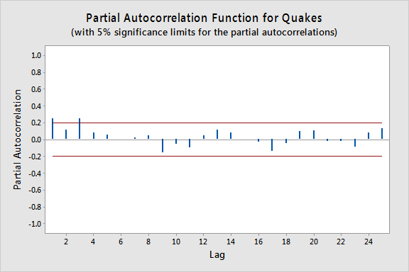
The plot below gives a plot of the PACF (partial autocorrelation function), which can be interpreted to mean that a third-order autoregression may be warranted since there are notable partial autocorrelations for lags 1 and 3.

The next step is to do a multiple linear regression with number of quakes as the response variable and lag-1, lag-2, and lag-3 quakes as the predictor variables. In the results below we see that the lag-3 predictor is significant at the 0.05 level (and the lag-1 predictor p-value is also relatively small).